Fig.2C-D. In silico estimates of mtDNA global structure

workflowr

• Summary
• Checks
• Past versions

Last updated: 2023-04-05

Checks: 7 0

Knit directory: GlobalStructure/

This reproducible R Markdown analysis was created with workflowr (version 1.7.0). The Checks tab describes the reproducibility checks that were applied when the results were created. The Past versions tab lists the development history.

---

R Markdown file: up-to-date

Great! Since the R Markdown file has been committed to the Git repository, you know the exact version of the code that produced these results.

Environment: empty

Great job! The global environment was empty. Objects defined in the global environment can affect the analysis in your R Markdown file in unknown ways. For reproduciblity it’s best to always run the code in an empty environment.

Seed: set.seed(20230404)

The command set.seed(20230404) was run prior to running the code in the R Markdown file. Setting a seed ensures that any results that rely on randomness, e.g. subsampling or permutations, are reproducible.

Session information: recorded

Great job! Recording the operating system, R version, and package versions is critical for reproducibility.

Cache: none

Nice! There were no cached chunks for this analysis, so you can be confident that you successfully produced the results during this run.

File paths: relative

Great job! Using relative paths to the files within your workflowr project makes it easier to run your code on other machines.

Repository version: baf2fd4

Great! You are using Git for version control. Tracking code development and connecting the code version to the results is critical for reproducibility.

The results in this page were generated with repository version baf2fd4. See the Past versions tab to see a history of the changes made to the R Markdown and HTML files.

Note that you need to be careful to ensure that all relevant files for the analysis have been committed to Git prior to generating the results (you can use wflow_publish or wflow_git_commit). workflowr only checks the R Markdown file, but you know if there are other scripts or data files that it depends on. Below is the status of the Git repository when the results were generated:

Ignored files:
    Ignored:    .Rproj.user/
    Ignored:    1_Raw/.DS_Store
    Ignored:    2_Derived/.DS_Store
    Ignored:    3_Results/.DS_Store
    Ignored:    renv/library/
    Ignored:    renv/staging/

Unstaged changes:
    Modified:   3_Results/violin_rep_center_release.pdf
    Modified:   3_Results/violin_rep_flanked_length_release.pdf

Note that any generated files, e.g. HTML, png, CSS, etc., are not included in this status report because it is ok for generated content to have uncommitted changes.

---

These are the previous versions of the repository in which changes were made to the R Markdown (analysis/figure_2cd.Rmd) and HTML (docs/figure_2cd.html) files. If you’ve configured a remote Git repository (see ?wflow_git_remote), click on the hyperlinks in the table below to view the files as they were in that past version.

File	Version	Author	Date	Message
Rmd	baf2fd4	Evgenii O. Tretiakov	2023-04-05	Start workflowr project.

---

1: READ microhomology from pair-wise alignments

homol <- read.table(
  here(data_dir, "HeatMaps/100x100.csv") %>%
    normalizePath(),
  sep = ";",
  header = TRUE
)
row.names(homol) <- homol$X
homol <- homol[, -1]
# make long vertical table from the matrix
for (i in seq_len(nrow(homol))) {
  for (j in seq_len(ncol(homol))) {
    # i  = 2; j = 1
    FirstWindow <- as.character(row.names(homol)[i])
    SecondWindow <- as.character(names(homol)[j])
    Score <- as.numeric(homol[i, j])
    OneLine <- data.frame(FirstWindow, SecondWindow, Score)
    if (i == 1 & j == 1) {
      Final <- OneLine
    }
    if (i > 1 | j > 1) {
      Final <- rbind(Final, OneLine)
    }
  }
}


Final$FirstWindow <- as.numeric(as.character(Final$FirstWindow))
Final$SecondWindow <- gsub("X", "", Final$SecondWindow) %>% as.numeric()

nrow(Final)

[1] 10000

Final <- Final[Final$FirstWindow > Final$SecondWindow, ]
nrow(Final)

[1] 4950

MicroHomology <- Final

2: READ density of direct repeats per window

DirectRepDensity <-
  here(
    data_dir, 
    "HeatMaps/Link_matrix_direct_major_activ_left.csv") %>%
  normalizePath() %>%
  read.table(
    sep = ";",
    header = TRUE
  )
DirectRepDensity <- DirectRepDensity[, -1]

# make long vertical table from the matrix
for (i in seq_len(nrow(DirectRepDensity))) {
  for (j in seq_len(ncol(DirectRepDensity))) {
    # i  = 2; j = 1
    FirstWindow <- as.character(row.names(DirectRepDensity)[i])
    SecondWindow <- as.character(names(DirectRepDensity)[j])
    Score <- as.numeric(DirectRepDensity[i, j])
    OneLine <- data.frame(FirstWindow, SecondWindow, Score)
    if (i == 1 & j == 1) {
      Final <- OneLine
    }
    if (i > 1 | j > 1) {
      Final <- rbind(Final, OneLine)
    }
  }
}


Final$FirstWindow <- as.numeric(as.character(Final$FirstWindow))
Final$SecondWindow <- gsub("X", "", Final$SecondWindow) %>% as.numeric()

nrow(Final)

[1] 10000

Final <- Final[Final$FirstWindow > Final$SecondWindow, ]
nrow(Final)

[1] 4950

DirectRepDensity <- Final

3: correlate MicroHomology and DirectRepDensity, derive HomologyAndRepeats dataset

DirectRepDensity <- DirectRepDensity[
  order(DirectRepDensity$FirstWindow, DirectRepDensity$SecondWindow),
]

MicroHomology <- MicroHomology[
  order(MicroHomology$FirstWindow, MicroHomology$SecondWindow),
]
pspearman::spearman.test(
  DirectRepDensity$Score,
  MicroHomology$Score
)

    Spearman's rank correlation rho

data:  DirectRepDensity$Score and MicroHomology$Score
S = 1.8841e+10, p-value = 1.707e-06
alternative hypothesis: true rho is not equal to 0
sample estimates:
       rho 
0.06796994 

nrow(DirectRepDensity) # 4950

[1] 4950

pspearman::spearman.test(
  DirectRepDensity[DirectRepDensity$Score > 0, ]$Score,
  MicroHomology[DirectRepDensity$Score > 0, ]$Score
)

    Spearman's rank correlation rho

data:  DirectRepDensity[DirectRepDensity$Score > 0, ]$Score and MicroHomology[DirectRepDensity$Score > 0, ]$Score
S = 1424127962, p-value = 0.006126
alternative hypothesis: true rho is not equal to 0
sample estimates:
       rho 
0.05998883 

HomologyAndRepeats <- data.frame(
  DirectRepDensity$FirstWindow,
  DirectRepDensity$SecondWindow,
  DirectRepDensity$Score,
  MicroHomology$Score
)
names(HomologyAndRepeats) <- c(
  "FirstWindow",
  "SecondWindow",
  "DirectRepeatsDensity",
  "MicroHomologyScore"
)

4: READ MITOBREAK AND FILTER (KEEP ONLY MAJOR ARC DELETIONS):

breaks <- read.table(
  here(raw_dir, "MitoBreakDB_12122019.csv") %>%
    normalizePath(),
  sep = ",",
  header = TRUE
)
breaks$X5..breakpoint <- as.numeric(as.character(breaks$X5..breakpoint))
summary(breaks$X5..breakpoint)

   Min. 1st Qu.  Median    Mean 3rd Qu.    Max.    NA's 
     83    6165    7668    7135    8562   16266       1 

breaks$X3..breakpoint <- as.numeric(as.character(breaks$X3..breakpoint))
summary(breaks$X3..breakpoint)

   Min. 1st Qu.  Median    Mean 3rd Qu.    Max.    NA's 
     24   13787   15075   14349   16035   16599       1 

breaks <- breaks[!is.na(breaks$X3..breakpoint) &
                   !is.na(breaks$X5..breakpoint), ]

breaks$FirstWindowBreakpoint <- breaks$X3..breakpoint
breaks$SecondWindowBreakpoint <- breaks$X5..breakpoint
breaks <- breaks[breaks$FirstWindowBreakpoint > 5781 &
                   breaks$FirstWindowBreakpoint < 16569 &
                   breaks$SecondWindowBreakpoint > 5781 &
                   breaks$SecondWindowBreakpoint < 16569, ]
# can make it better!! take in ot account 0-100?
# OH: 110-441
# OL: 5721-5781

HomologyAndRepeats$Deletion <- 0
for (i in seq_len(nrow(HomologyAndRepeats))) {
  # i = 1
  FirstWindow <- HomologyAndRepeats$FirstWindow[i]
  SecondWindow <- HomologyAndRepeats$SecondWindow[i]
  TempBreaks <- breaks[breaks$FirstWindowBreakpoint >= FirstWindow &
                         breaks$FirstWindowBreakpoint < (FirstWindow + 100) &
                         breaks$SecondWindowBreakpoint >= SecondWindow &
                         breaks$SecondWindowBreakpoint < (SecondWindow + 100), ]
  if (nrow(TempBreaks) > 0) {
    HomologyAndRepeats$Deletion[i] <- 1
  }
}

table(HomologyAndRepeats$Deletion)

   0    1 
4466  484 

skimr::skim(HomologyAndRepeats)

Data summary

Name	HomologyAndRepeats
Number of rows	4950
Number of columns	5
_______________________
Column type frequency:
numeric	5
________________________
Group variables	None

Variable type: numeric

skim_variable	n_missing	complete_rate	mean	sd	p0	p25	p50	p75	p100	hist
FirstWindow	0	1	12533.33	2345.21	6000	10900	12900	14500	15800	▁▃▅▆▇
SecondWindow	0	1	9166.67	2345.21	5900	7200	8800	10800	15700	▇▆▅▃▁
DirectRepeatsDensity	0	1	5.72	7.74	0	0	0	10	57	▇▁▁▁▁
MicroHomologyScore	0	1	90.09	17.27	27	79	89	101	160	▁▅▇▂▁
Deletion	0	1	0.10	0.30	0	0	0	0	1	▇▁▁▁▁

a <-
  glm(
    HomologyAndRepeats$Deletion ~ HomologyAndRepeats$DirectRepeatsDensity + HomologyAndRepeats$MicroHomologyScore,
    family = binomial
  )
summary(a)

Call:
glm(formula = HomologyAndRepeats$Deletion ~ HomologyAndRepeats$DirectRepeatsDensity + 
    HomologyAndRepeats$MicroHomologyScore, family = binomial)

Deviance Residuals: 
    Min       1Q   Median       3Q      Max  
-0.7475  -0.4768  -0.4359  -0.3951   2.5114  

Coefficients:
                                         Estimate Std. Error z value Pr(>|z|)
(Intercept)                             -3.693239   0.260347 -14.186  < 2e-16
HomologyAndRepeats$DirectRepeatsDensity  0.003526   0.006049   0.583     0.56
HomologyAndRepeats$MicroHomologyScore    0.015763   0.002729   5.776 7.63e-09
                                           
(Intercept)                             ***
HomologyAndRepeats$DirectRepeatsDensity    
HomologyAndRepeats$MicroHomologyScore   ***
---
Signif. codes:  0 '***' 0.001 '**' 0.01 '*' 0.05 '.' 0.1 ' ' 1

(Dispersion parameter for binomial family taken to be 1)

    Null deviance: 3169.7  on 4949  degrees of freedom
Residual deviance: 3135.5  on 4947  degrees of freedom
AIC: 3141.5

Number of Fisher Scoring iterations: 5

ggstatsplot::ggcoefstats(a)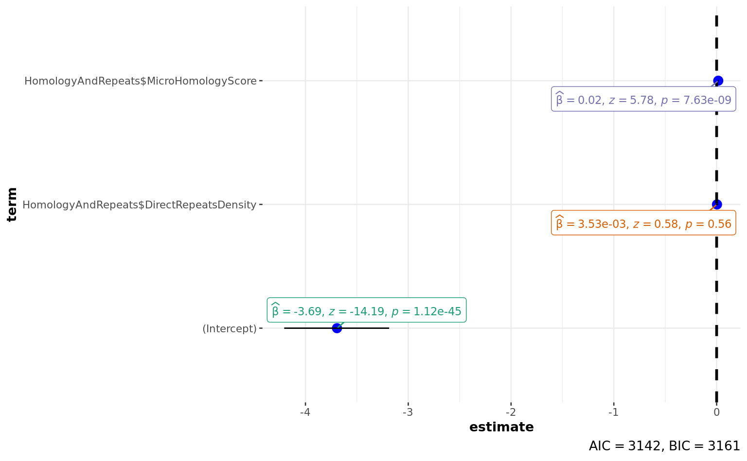

broom::tidy(a)

broom::glance(a)

a <-
  glm(
    HomologyAndRepeats$Deletion ~ scale(HomologyAndRepeats$MicroHomologyScore),
    family = binomial
  )
summary(a)

Call:
glm(formula = HomologyAndRepeats$Deletion ~ scale(HomologyAndRepeats$MicroHomologyScore), 
    family = binomial)

Deviance Residuals: 
    Min       1Q   Median       3Q      Max  
-0.7445  -0.4746  -0.4368  -0.3956   2.5063  

Coefficients:
                                             Estimate Std. Error z value
(Intercept)                                  -2.25264    0.04914 -45.838
scale(HomologyAndRepeats$MicroHomologyScore)  0.27442    0.04697   5.843
                                             Pr(>|z|)    
(Intercept)                                   < 2e-16 ***
scale(HomologyAndRepeats$MicroHomologyScore) 5.13e-09 ***
---
Signif. codes:  0 '***' 0.001 '**' 0.01 '*' 0.05 '.' 0.1 ' ' 1

(Dispersion parameter for binomial family taken to be 1)

    Null deviance: 3169.7  on 4949  degrees of freedom
Residual deviance: 3135.9  on 4948  degrees of freedom
AIC: 3139.9

Number of Fisher Scoring iterations: 5

ggstatsplot::ggcoefstats(a)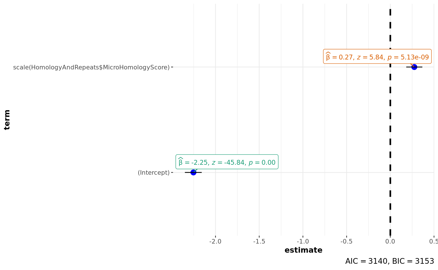

broom::tidy(a)

broom::glance(a)

may be add perfect repeats of Orlov - yes or no for each deletion? and see, if microhomology still important?

5: READ GLOBAL FOLDING:

GlobalFolding <-
  here(
    data_dir,
    "HeatMaps/Link_matrix1000_major.csv") %>%
  normalizePath() %>%
  read.table(
    sep = ";",
    header = TRUE
  )
row.names(GlobalFolding) <- GlobalFolding$X
GlobalFolding <- GlobalFolding[, -1]

# make long vertical table from the matrix
for (i in seq_len(nrow(GlobalFolding))) {
  for (j in seq_len(ncol(GlobalFolding))) {
    # i  = 2; j = 1
    FirstWindow <- as.character(row.names(GlobalFolding)[i])
    SecondWindow <- as.character(names(GlobalFolding)[j])
    Score <- as.numeric(GlobalFolding[i, j])
    OneLine <- data.frame(FirstWindow, SecondWindow, Score)
    if (i == 1 & j == 1) {
      Final <- OneLine
    }
    if (i > 1 | j > 1) {
      Final <- rbind(Final, OneLine)
    }
  }
}

## the matrix is symmetric - I need to keep only one triangle: X>Y (don't need also diagonal, which is noizy and bold)
Final$FirstWindow <- as.numeric(as.character(Final$FirstWindow))
Final$SecondWindow <- gsub("X", "", Final$SecondWindow) %>% as.numeric()

nrow(Final)

[1] 289

Final <- Final[Final$FirstWindow > Final$SecondWindow, ]
nrow(Final)

[1] 136

GlobalFolding1000 <- Final
GlobalFolding1000 <- GlobalFolding1000[order(
  GlobalFolding1000$FirstWindow,
  GlobalFolding1000$SecondWindow
), ]
names(GlobalFolding1000) <- c(
  "FirstWindowWholeKbRes",
  "SecondWindowWholeKbRes",
  "GlobalFolding1000Score"
)

5.1: UPDATE GLOBAL FOLDING WITH WINDOW = 100 bp: (it automaticaly rewrites the GlobalFolding matrix from the previous point 5)

GlobalFolding <-
  here(
    data_dir,
    "HeatMaps/Link_matrix100hydra_major.csv") %>%
  normalizePath() %>%
  read.table(
    sep = ";",
    header = TRUE
  )
row.names(GlobalFolding) <- GlobalFolding$X
GlobalFolding <- GlobalFolding[, -1]

# make long vertical table from the matrix
for (i in seq_len(nrow(GlobalFolding))) {
  for (j in seq_len(ncol(GlobalFolding))) {
    # i  = 2; j = 1
    FirstWindow <- as.character(row.names(GlobalFolding)[i])
    SecondWindow <- as.character(names(GlobalFolding)[j])
    Score <- as.numeric(GlobalFolding[i, j])
    OneLine <- data.frame(FirstWindow, SecondWindow, Score)
    if (i == 1 & j == 1) {
      Final <- OneLine
    }
    if (i > 1 | j > 1) {
      Final <- rbind(Final, OneLine)
    }
  }
}


Final$FirstWindow <- as.numeric(as.character(Final$FirstWindow))
Final$SecondWindow <- gsub("X", "", Final$SecondWindow) %>% as.numeric()

nrow(Final)

[1] 27556

Final <- Final[Final$FirstWindow > Final$SecondWindow, ]
nrow(Final)

[1] 13695

# Should we delete bold diagonal or erase it to zeroes??? If delete, dimension will be decreased - try this. delete 5 windows next to diagonal (500)
nrow(Final)

[1] 13695

Final <- Final[Final$FirstWindow > Final$SecondWindow + 1000, ]
nrow(Final) # 500 or 1000!!!!!! similarly good results but 1000 is a bit better

[1] 12090

GlobalFolding <- Final
GlobalFolding <- GlobalFolding[order(GlobalFolding$FirstWindow, GlobalFolding$SecondWindow), ]
names(GlobalFolding)[3] <- c("GlobalFoldingScore")

pltHeatmap_gFolding_sw100 <-
  here(data_dir, "HeatMaps/Link_matrix100hydra_major.csv") %>%
  read.table(
    sep = ";",
    header = TRUE
  ) %>%
  gather(-X,
         key = "SecondWindow",
         value = "Score"
  ) %>%
  rename(FirstWindow = X) %>%
  mutate(SecondWindow = stringr::str_extract(
    SecondWindow,
    "\\d+"
  ) %>%
    as.integer()) %>%
  filter(
    FirstWindow >= 5950,
    SecondWindow >= 5950
  ) %>%
  tibble() %>%
  ggplot(aes(
    x = FirstWindow,
    y = SecondWindow,
    fill = Score
  )) +
  geom_tile() +
  scale_y_reverse() +
  scale_fill_viridis_c(option = "D", direction = -1) +
  theme_bw(base_size = 18)

cowplot::save_plot(
  plot = pltHeatmap_gFolding_sw100,
  base_height = 8.316,
  base_width = 11.594,
  file = normalizePath(
    file.path(plots_dir, "heatmap_global_folding_sw100.pdf")
  )
)

pltHeatmap_gFolding_sw100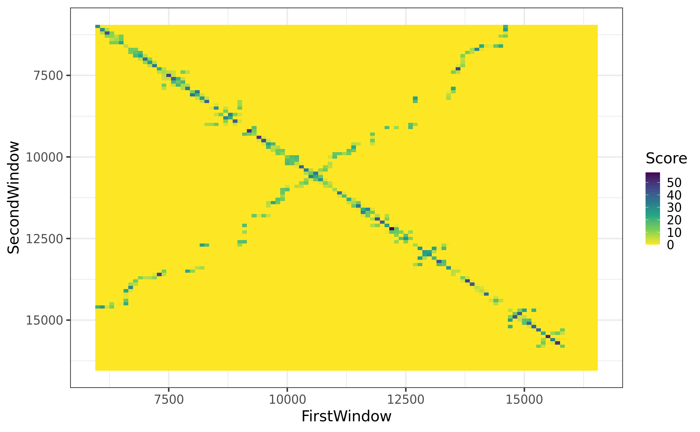

folding_df <-
  here(
    data_dir,
    "HeatMaps/Link_matrix100hydra_major.csv") %>%
  read.table(
    sep = ";",
    header = TRUE
  ) %>%
  gather(-X,
         key = "SecondWindow",
         value = "Score"
  ) %>%
  rename(FirstWindow = X) %>%
  mutate(SecondWindow = stringr::str_extract(
    SecondWindow,
    "\\d+"
  ) %>%
    as.integer()) %>%
  filter(
    FirstWindow >= 5950,
    SecondWindow >= 5950
  ) %>%
  tibble()

GlobalFolding - is the whole genome without bold diagonal, not only the major arc!! Keep only major arc in downstream analyses. (will do it when merge with InvRepDens)

5.2: STABILITY OF DUPLEXES

stblt_df <-
  read.csv(here(
    data_dir,
    "HeatMaps/duplex-stablility_100x100.mtrx"),
    sep = ";",
    row.names = 1
  ) %>% .[, -dim(.)[2]]
# I don't know why coordinates aren't equal so I match them first
all((dimnames(stblt_df)[[2]] |> str_remove("X")) %in% dimnames(stblt_df)[[1]]) # TRUE

[1] TRUE

all(dimnames(stblt_df)[[1]] %in% (dimnames(stblt_df)[[2]] |> str_remove("X"))) # FALSE

[1] FALSE

dimnames(stblt_df)[[2]] <-
  dimnames(stblt_df)[[1]][match(
    dimnames(stblt_df)[[2]] |> str_remove("X"),
    dimnames(stblt_df)[[1]]
  )]
# stblt_df <- stblt_df[dimnames(stblt_df)[[2]], ]
# dim(stblt_df) # 108 x 108

stblt_mtrx <- as.matrix(stblt_df)
dimnames(stblt_mtrx) <- list(
  x = as.integer(dimnames(stblt_df)[[1]]),
  y = as.integer(dimnames(stblt_df)[[2]])
)
stblt_plot2d <-
  melt(stblt_mtrx, value.name = "duplexes_stability") |>
  mutate(x = x + 19, y = y + 19)
gg_stblt <-
  ggplot(
    stblt_plot2d,
    aes(x, y,
        z = duplexes_stability,
        fill = duplexes_stability
    )
  )
gg_duplexes_stability <- gg_stblt + geom_raster(interpolate = TRUE)
gg_duplexes_stability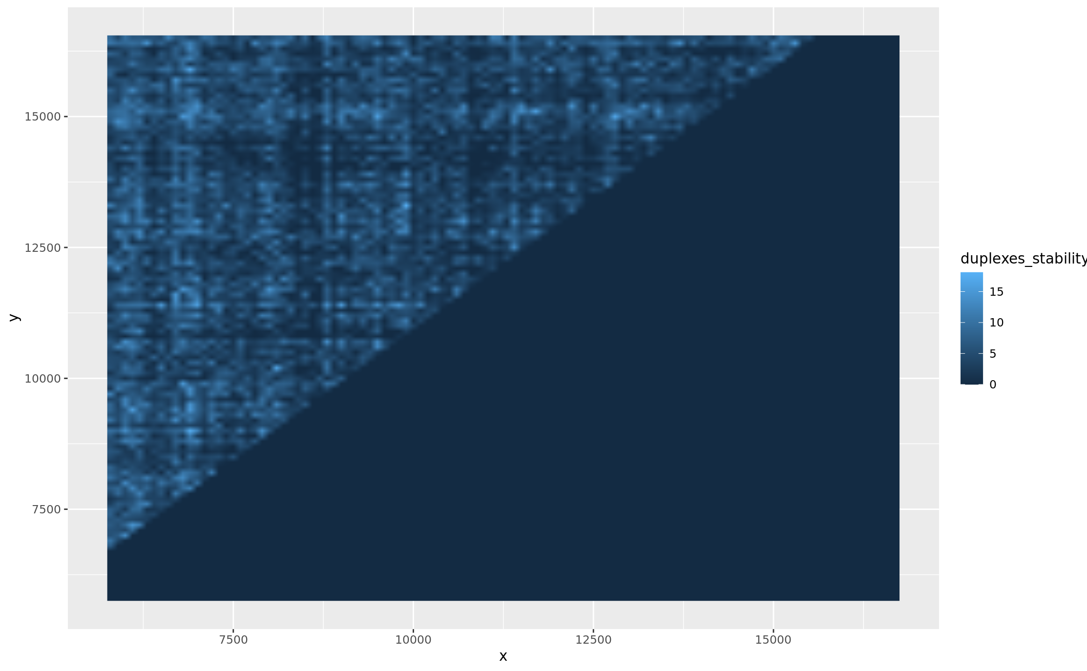

Article version Figure 2D: Heatmap merged Stability of duplexes and Global folding scores

bind_df <-
  inner_join(
    folding_df, stblt_plot2d,
    by = c(
      "FirstWindow" = "x",
      "SecondWindow" = "y"
    ),
    keep = FALSE
  ) %>%
  asymmetrise(
    .,
    FirstWindow,
    SecondWindow
  )

gg_bind <-
  ggplot(
    bind_df,
    aes(
      x = FirstWindow,
      y = SecondWindow
    )
  ) +
  geom_asymmat(aes(
    fill_br = duplexes_stability,
    fill_tl = Score
  )) +
  scale_fill_br_gradientn(
    colours = viridis::viridis(2000)[250:2000],
    na.value = "white",
    guide = guide_colourbar(
      direction = "horizontal",
      order = 1,
      title.position = "top",
      barwidth = 10, barheight = 1
    )
  ) +
  scale_fill_tl_distiller(
    type = "div",
    palette = "RdYlBu",
    direction = 1,
    na.value = "white",
    guide = guide_colourbar(
      direction = "horizontal",
      order = 2,
      title.position = "top",
      barwidth = 10, barheight = 1
    )
  ) +
  labs(
    fill_tl = "bottom-left Stability of duplexes",
    fill_br = "top-right Global folding",
    title = "Model of mtDNA structural stability"
  ) +
  theme_bw() +
  theme(
    axis.title = element_blank(),
    plot.title = element_text(hjust = 0.5),
    panel.background = element_rect(fill = "white"),
    panel.grid = element_blank(),
    legend.position = "bottom",
    legend.box = "horizontal"
  )

cowplot::save_plot(
  plot = gg_bind,
  base_height = 8.316,
  base_asp = 0.9,
  file = here(plots_dir, "heatmap_folding_stability.svg")
)

gg_bind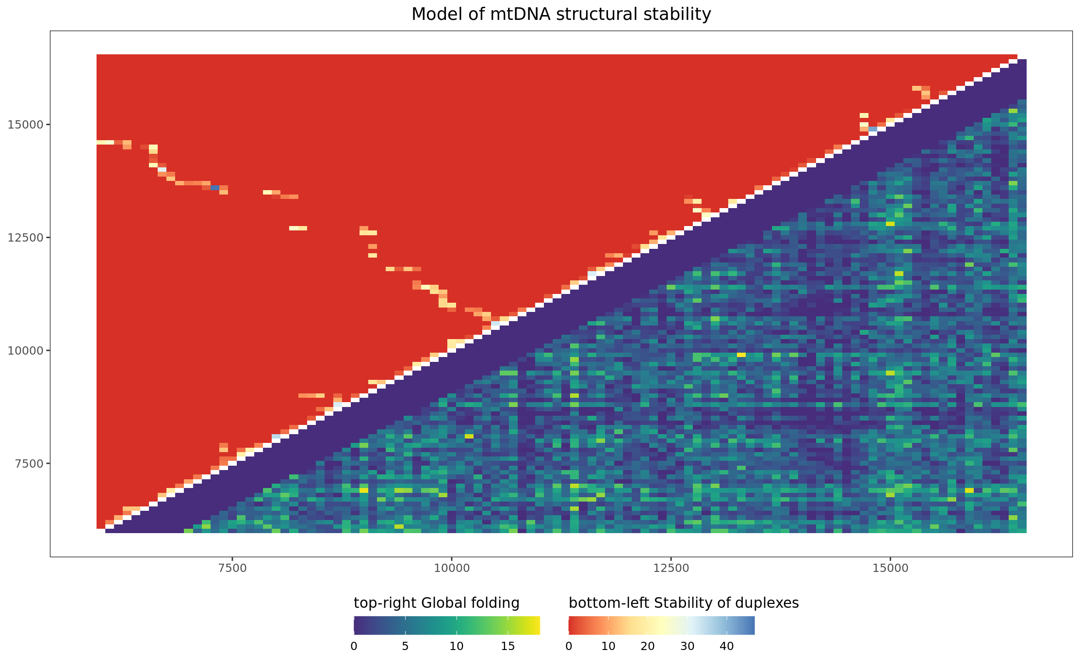

6: READ INVERTED REPEATS WITH STEP 1000

InvRepDens <-
  here(
    data_dir,
    "HeatMaps/Link_matrix_1000_invert_major_activ_left.csv") %>%
  normalizePath() %>%
  read.table(
    sep = ";",
    header = TRUE
  )
row.names(InvRepDens) <- InvRepDens$X
InvRepDens <- InvRepDens[, -1]

# make long vertical table from the matrix
for (i in seq_len(nrow(InvRepDens))) {
  for (j in seq_len(ncol(InvRepDens))) {
    # i  = 2; j = 1
    FirstWindow <- as.character(row.names(InvRepDens)[i])
    SecondWindow <- as.character(names(InvRepDens)[j])
    Score <- as.numeric(InvRepDens[i, j])
    OneLine <- data.frame(FirstWindow, SecondWindow, Score)
    if (i == 1 & j == 1) {
      Final <- OneLine
    }
    if (i > 1 | j > 1) {
      Final <- rbind(Final, OneLine)
    }
  }
}


Final$FirstWindow <- as.numeric(as.character(Final$FirstWindow))
Final$SecondWindow <- gsub("X", "", Final$SecondWindow) %>% as.numeric()

nrow(Final)

[1] 289

Final <- Final[Final$FirstWindow > Final$SecondWindow, ]
nrow(Final)

[1] 136

InvRepDens <- Final
InvRepDens <- InvRepDens[order(InvRepDens$FirstWindow, InvRepDens$SecondWindow), ]

6.1: UPDATE INVERTED REPEATS WITH STEP 100 bp (it automatically rewrites InvRepDens from previous point 6)

InvRepDens <-
  here("2_Derived/HeatMaps/Link_matrix_invert_major_activ_left.modified.csv") %>%
  normalizePath() %>%
  read.table(
    sep = "\t",
    header = TRUE,
    row.names = 1
  ) # , row.names = NULL)

# make long vertical table from the matrix
for (i in seq_len(nrow(InvRepDens))) {
  for (j in seq_len(ncol(InvRepDens))) {
    # i  = 2; j = 1
    FirstWindow <- as.character(row.names(InvRepDens)[i])
    SecondWindow <- as.character(names(InvRepDens)[j])
    Score <- as.numeric(InvRepDens[i, j])
    OneLine <- data.frame(FirstWindow, SecondWindow, Score)
    if (i == 1 & j == 1) {
      Final <- OneLine
    }
    if (i > 1 | j > 1) {
      Final <- rbind(Final, OneLine)
    }
  }
}


Final$FirstWindow <- as.numeric(as.character(Final$FirstWindow))
Final$SecondWindow <- gsub("X", "", Final$SecondWindow) %>% as.numeric()

nrow(Final)

[1] 10000

Final <- Final[Final$FirstWindow > Final$SecondWindow, ]
nrow(Final)

[1] 4950

InvRepDens <- Final
InvRepDens <- InvRepDens[order(InvRepDens$FirstWindow, InvRepDens$SecondWindow), ]

names(InvRepDens)[3] <- c("InvRepDensScore")
skimr::skim(InvRepDens)

Data summary

Name	InvRepDens
Number of rows	4950
Number of columns	3
_______________________
Column type frequency:
numeric	3
________________________
Group variables	None

Variable type: numeric

skim_variable	n_missing	complete_rate	mean	sd	p0	p25	p50	p75	p100	hist
FirstWindow	0	1	12533.33	2345.21	6000	10900	12900	14500	15800	▁▃▅▆▇
SecondWindow	0	1	9166.67	2345.21	5900	7200	8800	10800	15700	▇▆▅▃▁
InvRepDensScore	0	1	1.42	3.88	0	0	0	0	31	▇▁▁▁▁

7: CORRELATE InvRepDens\(Score and GlobalFolding\)Score

• weak positive!

merged <- merge(InvRepDens, GlobalFolding, by = c("FirstWindow", "SecondWindow"))
summary(merged$FirstWindow) # diag 500: 6500 15800; diag 1000: 7000 - 15800

   Min. 1st Qu.  Median    Mean 3rd Qu.    Max. 
   7000   11400   13200   12867   14700   15800 

summary(merged$SecondWindow) # diag 500: 5900 15200; diag 1000: 5900 14700

   Min. 1st Qu.  Median    Mean 3rd Qu.    Max. 
   5900    7000    8500    8833   10300   14700 

skimr::skim(merged)

Data summary

Name	merged
Number of rows	4005
Number of columns	4
_______________________
Column type frequency:
numeric	4
________________________
Group variables	None

Variable type: numeric

skim_variable	n_missing	complete_rate	mean	sd	p0	p25	p50	p75	p100	hist
FirstWindow	0	1	12866.67	2109.50	7000	11400	13200	14700	15800	▁▃▅▆▇
SecondWindow	0	1	8833.33	2109.50	5900	7000	8500	10300	14700	▇▆▅▃▁
InvRepDensScore	0	1	1.39	3.81	0	0	0	0	31	▇▁▁▁▁
GlobalFoldingScore	0	1	0.16	1.74	0	0	0	0	47	▇▁▁▁▁

pspearman::spearman.test(merged$InvRepDensScore, merged$GlobalFoldingScore)

    Spearman's rank correlation rho

data:  merged$InvRepDensScore and merged$GlobalFoldingScore
S = 1.0177e+10, p-value = 0.001745
alternative hypothesis: true rho is not equal to 0
sample estimates:
       rho 
0.04945796 

nrow(merged) # 4005

[1] 4005

8: ADD InfinitySign parameter into HomologyAndRepeats dataset (13 - 16 kb vs 6-9 kb):

HomologyAndRepeats$InfinitySign <- 0
for (i in seq_len(nrow(HomologyAndRepeats))) {
  if (HomologyAndRepeats$FirstWindow[i] >= 13000 &
      HomologyAndRepeats$FirstWindow[i] <= 16000 &
      HomologyAndRepeats$SecondWindow[i] >= 6000 &
      HomologyAndRepeats$SecondWindow[i] <= 9000) {
    HomologyAndRepeats$InfinitySign[i] <- 1
  }
}
janitor::tabyl(HomologyAndRepeats$InfinitySign)

janitor::tabyl(HomologyAndRepeats, Deletion, InfinitySign)

sjmisc::frq(HomologyAndRepeats)

FirstWindow <numeric> 
# total N=4950 valid N=4950 mean=12533.33 sd=2345.21

Value |  N | Raw % | Valid % | Cum. %
-------------------------------------
 6000 |  1 |  0.02 |    0.02 |   0.02
 6100 |  2 |  0.04 |    0.04 |   0.06
 6200 |  3 |  0.06 |    0.06 |   0.12
 6300 |  4 |  0.08 |    0.08 |   0.20
 6400 |  5 |  0.10 |    0.10 |   0.30
 6500 |  6 |  0.12 |    0.12 |   0.42
 6600 |  7 |  0.14 |    0.14 |   0.57
 6700 |  8 |  0.16 |    0.16 |   0.73
 6800 |  9 |  0.18 |    0.18 |   0.91
 6900 | 10 |  0.20 |    0.20 |   1.11
 7000 | 11 |  0.22 |    0.22 |   1.33
 7100 | 12 |  0.24 |    0.24 |   1.58
 7200 | 13 |  0.26 |    0.26 |   1.84
 7300 | 14 |  0.28 |    0.28 |   2.12
 7400 | 15 |  0.30 |    0.30 |   2.42
 7500 | 16 |  0.32 |    0.32 |   2.75
 7600 | 17 |  0.34 |    0.34 |   3.09
 7700 | 18 |  0.36 |    0.36 |   3.45
 7800 | 19 |  0.38 |    0.38 |   3.84
 7900 | 20 |  0.40 |    0.40 |   4.24
 8000 | 21 |  0.42 |    0.42 |   4.67
 8100 | 22 |  0.44 |    0.44 |   5.11
 8200 | 23 |  0.46 |    0.46 |   5.58
 8300 | 24 |  0.48 |    0.48 |   6.06
 8400 | 25 |  0.51 |    0.51 |   6.57
 8500 | 26 |  0.53 |    0.53 |   7.09
 8600 | 27 |  0.55 |    0.55 |   7.64
 8700 | 28 |  0.57 |    0.57 |   8.20
 8800 | 29 |  0.59 |    0.59 |   8.79
 8900 | 30 |  0.61 |    0.61 |   9.39
 9000 | 31 |  0.63 |    0.63 |  10.02
 9100 | 32 |  0.65 |    0.65 |  10.67
 9200 | 33 |  0.67 |    0.67 |  11.33
 9300 | 34 |  0.69 |    0.69 |  12.02
 9400 | 35 |  0.71 |    0.71 |  12.73
 9500 | 36 |  0.73 |    0.73 |  13.45
 9600 | 37 |  0.75 |    0.75 |  14.20
 9700 | 38 |  0.77 |    0.77 |  14.97
 9800 | 39 |  0.79 |    0.79 |  15.76
 9900 | 40 |  0.81 |    0.81 |  16.57
10000 | 41 |  0.83 |    0.83 |  17.39
10100 | 42 |  0.85 |    0.85 |  18.24
10200 | 43 |  0.87 |    0.87 |  19.11
10300 | 44 |  0.89 |    0.89 |  20.00
10400 | 45 |  0.91 |    0.91 |  20.91
10500 | 46 |  0.93 |    0.93 |  21.84
10600 | 47 |  0.95 |    0.95 |  22.79
10700 | 48 |  0.97 |    0.97 |  23.76
10800 | 49 |  0.99 |    0.99 |  24.75
10900 | 50 |  1.01 |    1.01 |  25.76
11000 | 51 |  1.03 |    1.03 |  26.79
11100 | 52 |  1.05 |    1.05 |  27.84
11200 | 53 |  1.07 |    1.07 |  28.91
11300 | 54 |  1.09 |    1.09 |  30.00
11400 | 55 |  1.11 |    1.11 |  31.11
11500 | 56 |  1.13 |    1.13 |  32.24
11600 | 57 |  1.15 |    1.15 |  33.39
11700 | 58 |  1.17 |    1.17 |  34.57
11800 | 59 |  1.19 |    1.19 |  35.76
11900 | 60 |  1.21 |    1.21 |  36.97
12000 | 61 |  1.23 |    1.23 |  38.20
12100 | 62 |  1.25 |    1.25 |  39.45
12200 | 63 |  1.27 |    1.27 |  40.73
12300 | 64 |  1.29 |    1.29 |  42.02
12400 | 65 |  1.31 |    1.31 |  43.33
12500 | 66 |  1.33 |    1.33 |  44.67
12600 | 67 |  1.35 |    1.35 |  46.02
12700 | 68 |  1.37 |    1.37 |  47.39
12800 | 69 |  1.39 |    1.39 |  48.79
12900 | 70 |  1.41 |    1.41 |  50.20
13000 | 71 |  1.43 |    1.43 |  51.64
13100 | 72 |  1.45 |    1.45 |  53.09
13200 | 73 |  1.47 |    1.47 |  54.57
13300 | 74 |  1.49 |    1.49 |  56.06
13400 | 75 |  1.52 |    1.52 |  57.58
13500 | 76 |  1.54 |    1.54 |  59.11
13600 | 77 |  1.56 |    1.56 |  60.67
13700 | 78 |  1.58 |    1.58 |  62.24
13800 | 79 |  1.60 |    1.60 |  63.84
13900 | 80 |  1.62 |    1.62 |  65.45
14000 | 81 |  1.64 |    1.64 |  67.09
14100 | 82 |  1.66 |    1.66 |  68.75
14200 | 83 |  1.68 |    1.68 |  70.42
14300 | 84 |  1.70 |    1.70 |  72.12
14400 | 85 |  1.72 |    1.72 |  73.84
14500 | 86 |  1.74 |    1.74 |  75.58
14600 | 87 |  1.76 |    1.76 |  77.33
14700 | 88 |  1.78 |    1.78 |  79.11
14800 | 89 |  1.80 |    1.80 |  80.91
14900 | 90 |  1.82 |    1.82 |  82.73
15000 | 91 |  1.84 |    1.84 |  84.57
15100 | 92 |  1.86 |    1.86 |  86.42
15200 | 93 |  1.88 |    1.88 |  88.30
15300 | 94 |  1.90 |    1.90 |  90.20
15400 | 95 |  1.92 |    1.92 |  92.12
15500 | 96 |  1.94 |    1.94 |  94.06
15600 | 97 |  1.96 |    1.96 |  96.02
15700 | 98 |  1.98 |    1.98 |  98.00
15800 | 99 |  2.00 |    2.00 | 100.00
 <NA> |  0 |  0.00 |    <NA> |   <NA>

SecondWindow <numeric> 
# total N=4950 valid N=4950 mean=9166.67 sd=2345.21

Value |  N | Raw % | Valid % | Cum. %
-------------------------------------
 5900 | 99 |  2.00 |    2.00 |   2.00
 6000 | 98 |  1.98 |    1.98 |   3.98
 6100 | 97 |  1.96 |    1.96 |   5.94
 6200 | 96 |  1.94 |    1.94 |   7.88
 6300 | 95 |  1.92 |    1.92 |   9.80
 6400 | 94 |  1.90 |    1.90 |  11.70
 6500 | 93 |  1.88 |    1.88 |  13.58
 6600 | 92 |  1.86 |    1.86 |  15.43
 6700 | 91 |  1.84 |    1.84 |  17.27
 6800 | 90 |  1.82 |    1.82 |  19.09
 6900 | 89 |  1.80 |    1.80 |  20.89
 7000 | 88 |  1.78 |    1.78 |  22.67
 7100 | 87 |  1.76 |    1.76 |  24.42
 7200 | 86 |  1.74 |    1.74 |  26.16
 7300 | 85 |  1.72 |    1.72 |  27.88
 7400 | 84 |  1.70 |    1.70 |  29.58
 7500 | 83 |  1.68 |    1.68 |  31.25
 7600 | 82 |  1.66 |    1.66 |  32.91
 7700 | 81 |  1.64 |    1.64 |  34.55
 7800 | 80 |  1.62 |    1.62 |  36.16
 7900 | 79 |  1.60 |    1.60 |  37.76
 8000 | 78 |  1.58 |    1.58 |  39.33
 8100 | 77 |  1.56 |    1.56 |  40.89
 8200 | 76 |  1.54 |    1.54 |  42.42
 8300 | 75 |  1.52 |    1.52 |  43.94
 8400 | 74 |  1.49 |    1.49 |  45.43
 8500 | 73 |  1.47 |    1.47 |  46.91
 8600 | 72 |  1.45 |    1.45 |  48.36
 8700 | 71 |  1.43 |    1.43 |  49.80
 8800 | 70 |  1.41 |    1.41 |  51.21
 8900 | 69 |  1.39 |    1.39 |  52.61
 9000 | 68 |  1.37 |    1.37 |  53.98
 9100 | 67 |  1.35 |    1.35 |  55.33
 9200 | 66 |  1.33 |    1.33 |  56.67
 9300 | 65 |  1.31 |    1.31 |  57.98
 9400 | 64 |  1.29 |    1.29 |  59.27
 9500 | 63 |  1.27 |    1.27 |  60.55
 9600 | 62 |  1.25 |    1.25 |  61.80
 9700 | 61 |  1.23 |    1.23 |  63.03
 9800 | 60 |  1.21 |    1.21 |  64.24
 9900 | 59 |  1.19 |    1.19 |  65.43
10000 | 58 |  1.17 |    1.17 |  66.61
10100 | 57 |  1.15 |    1.15 |  67.76
10200 | 56 |  1.13 |    1.13 |  68.89
10300 | 55 |  1.11 |    1.11 |  70.00
10400 | 54 |  1.09 |    1.09 |  71.09
10500 | 53 |  1.07 |    1.07 |  72.16
10600 | 52 |  1.05 |    1.05 |  73.21
10700 | 51 |  1.03 |    1.03 |  74.24
10800 | 50 |  1.01 |    1.01 |  75.25
10900 | 49 |  0.99 |    0.99 |  76.24
11000 | 48 |  0.97 |    0.97 |  77.21
11100 | 47 |  0.95 |    0.95 |  78.16
11200 | 46 |  0.93 |    0.93 |  79.09
11300 | 45 |  0.91 |    0.91 |  80.00
11400 | 44 |  0.89 |    0.89 |  80.89
11500 | 43 |  0.87 |    0.87 |  81.76
11600 | 42 |  0.85 |    0.85 |  82.61
11700 | 41 |  0.83 |    0.83 |  83.43
11800 | 40 |  0.81 |    0.81 |  84.24
11900 | 39 |  0.79 |    0.79 |  85.03
12000 | 38 |  0.77 |    0.77 |  85.80
12100 | 37 |  0.75 |    0.75 |  86.55
12200 | 36 |  0.73 |    0.73 |  87.27
12300 | 35 |  0.71 |    0.71 |  87.98
12400 | 34 |  0.69 |    0.69 |  88.67
12500 | 33 |  0.67 |    0.67 |  89.33
12600 | 32 |  0.65 |    0.65 |  89.98
12700 | 31 |  0.63 |    0.63 |  90.61
12800 | 30 |  0.61 |    0.61 |  91.21
12900 | 29 |  0.59 |    0.59 |  91.80
13000 | 28 |  0.57 |    0.57 |  92.36
13100 | 27 |  0.55 |    0.55 |  92.91
13200 | 26 |  0.53 |    0.53 |  93.43
13300 | 25 |  0.51 |    0.51 |  93.94
13400 | 24 |  0.48 |    0.48 |  94.42
13500 | 23 |  0.46 |    0.46 |  94.89
13600 | 22 |  0.44 |    0.44 |  95.33
13700 | 21 |  0.42 |    0.42 |  95.76
13800 | 20 |  0.40 |    0.40 |  96.16
13900 | 19 |  0.38 |    0.38 |  96.55
14000 | 18 |  0.36 |    0.36 |  96.91
14100 | 17 |  0.34 |    0.34 |  97.25
14200 | 16 |  0.32 |    0.32 |  97.58
14300 | 15 |  0.30 |    0.30 |  97.88
14400 | 14 |  0.28 |    0.28 |  98.16
14500 | 13 |  0.26 |    0.26 |  98.42
14600 | 12 |  0.24 |    0.24 |  98.67
14700 | 11 |  0.22 |    0.22 |  98.89
14800 | 10 |  0.20 |    0.20 |  99.09
14900 |  9 |  0.18 |    0.18 |  99.27
15000 |  8 |  0.16 |    0.16 |  99.43
15100 |  7 |  0.14 |    0.14 |  99.58
15200 |  6 |  0.12 |    0.12 |  99.70
15300 |  5 |  0.10 |    0.10 |  99.80
15400 |  4 |  0.08 |    0.08 |  99.88
15500 |  3 |  0.06 |    0.06 |  99.94
15600 |  2 |  0.04 |    0.04 |  99.98
15700 |  1 |  0.02 |    0.02 | 100.00
 <NA> |  0 |  0.00 |    <NA> |   <NA>

DirectRepeatsDensity <numeric> 
# total N=4950 valid N=4950 mean=5.72 sd=7.74

Value |    N | Raw % | Valid % | Cum. %
---------------------------------------
    0 | 2863 | 57.84 |   57.84 |  57.84
    5 |    7 |  0.14 |    0.14 |  57.98
    6 |   30 |  0.61 |    0.61 |  58.59
    7 |   33 |  0.67 |    0.67 |  59.25
    8 |   33 |  0.67 |    0.67 |  59.92
    9 |   27 |  0.55 |    0.55 |  60.46
   10 |  838 | 16.93 |   16.93 |  77.39
   11 |  263 |  5.31 |    5.31 |  82.71
   12 |  157 |  3.17 |    3.17 |  85.88
   13 |  101 |  2.04 |    2.04 |  87.92
   14 |   36 |  0.73 |    0.73 |  88.65
   15 |   32 |  0.65 |    0.65 |  89.29
   16 |   26 |  0.53 |    0.53 |  89.82
   17 |   29 |  0.59 |    0.59 |  90.40
   18 |   29 |  0.59 |    0.59 |  90.99
   19 |   20 |  0.40 |    0.40 |  91.39
   20 |  119 |  2.40 |    2.40 |  93.80
   21 |   84 |  1.70 |    1.70 |  95.49
   22 |   46 |  0.93 |    0.93 |  96.42
   23 |   43 |  0.87 |    0.87 |  97.29
   24 |   31 |  0.63 |    0.63 |  97.92
   25 |   10 |  0.20 |    0.20 |  98.12
   26 |   13 |  0.26 |    0.26 |  98.38
   27 |    5 |  0.10 |    0.10 |  98.48
   28 |    7 |  0.14 |    0.14 |  98.63
   29 |    8 |  0.16 |    0.16 |  98.79
   30 |   10 |  0.20 |    0.20 |  98.99
   31 |    7 |  0.14 |    0.14 |  99.13
   32 |   10 |  0.20 |    0.20 |  99.33
   33 |    8 |  0.16 |    0.16 |  99.49
   34 |   10 |  0.20 |    0.20 |  99.70
   35 |    5 |  0.10 |    0.10 |  99.80
   36 |    1 |  0.02 |    0.02 |  99.82
   37 |    1 |  0.02 |    0.02 |  99.84
   38 |    1 |  0.02 |    0.02 |  99.86
   39 |    1 |  0.02 |    0.02 |  99.88
   41 |    1 |  0.02 |    0.02 |  99.90
   43 |    1 |  0.02 |    0.02 |  99.92
   44 |    2 |  0.04 |    0.04 |  99.96
   53 |    1 |  0.02 |    0.02 |  99.98
   57 |    1 |  0.02 |    0.02 | 100.00
 <NA> |    0 |  0.00 |    <NA> |   <NA>

MicroHomologyScore <numeric> 
# total N=4950 valid N=4950 mean=90.09 sd=17.27

Value |   N | Raw % | Valid % | Cum. %
--------------------------------------
   27 |   1 |  0.02 |    0.02 |   0.02
   32 |   1 |  0.02 |    0.02 |   0.04
   33 |   2 |  0.04 |    0.04 |   0.08
   35 |   2 |  0.04 |    0.04 |   0.12
   37 |   1 |  0.02 |    0.02 |   0.14
   40 |   2 |  0.04 |    0.04 |   0.18
   41 |   1 |  0.02 |    0.02 |   0.20
   42 |   3 |  0.06 |    0.06 |   0.26
   43 |   5 |  0.10 |    0.10 |   0.36
   44 |   3 |  0.06 |    0.06 |   0.42
   45 |   6 |  0.12 |    0.12 |   0.55
   46 |   2 |  0.04 |    0.04 |   0.59
   47 |   3 |  0.06 |    0.06 |   0.65
   48 |   3 |  0.06 |    0.06 |   0.71
   49 |   9 |  0.18 |    0.18 |   0.89
   50 |   4 |  0.08 |    0.08 |   0.97
   51 |   6 |  0.12 |    0.12 |   1.09
   52 |   3 |  0.06 |    0.06 |   1.15
   53 |   9 |  0.18 |    0.18 |   1.33
   54 |   4 |  0.08 |    0.08 |   1.41
   55 |  18 |  0.36 |    0.36 |   1.78
   56 |   5 |  0.10 |    0.10 |   1.88
   57 |  11 |  0.22 |    0.22 |   2.10
   58 |  23 |  0.46 |    0.46 |   2.57
   59 |  21 |  0.42 |    0.42 |   2.99
   60 |  22 |  0.44 |    0.44 |   3.43
   61 |  28 |  0.57 |    0.57 |   4.00
   62 |  31 |  0.63 |    0.63 |   4.63
   63 |  32 |  0.65 |    0.65 |   5.27
   64 |  44 |  0.89 |    0.89 |   6.16
   65 |  28 |  0.57 |    0.57 |   6.73
   66 |  34 |  0.69 |    0.69 |   7.41
   67 |  36 |  0.73 |    0.73 |   8.14
   68 |  55 |  1.11 |    1.11 |   9.25
   69 |  50 |  1.01 |    1.01 |  10.26
   70 |  65 |  1.31 |    1.31 |  11.58
   71 |  61 |  1.23 |    1.23 |  12.81
   72 |  71 |  1.43 |    1.43 |  14.24
   73 |  65 |  1.31 |    1.31 |  15.56
   74 |  73 |  1.47 |    1.47 |  17.03
   75 |  74 |  1.49 |    1.49 |  18.53
   76 |  90 |  1.82 |    1.82 |  20.34
   77 | 107 |  2.16 |    2.16 |  22.51
   78 | 111 |  2.24 |    2.24 |  24.75
   79 |  93 |  1.88 |    1.88 |  26.63
   80 | 105 |  2.12 |    2.12 |  28.75
   81 | 121 |  2.44 |    2.44 |  31.19
   82 | 125 |  2.53 |    2.53 |  33.72
   83 | 126 |  2.55 |    2.55 |  36.26
   84 | 121 |  2.44 |    2.44 |  38.71
   85 | 132 |  2.67 |    2.67 |  41.37
   86 | 114 |  2.30 |    2.30 |  43.68
   87 | 114 |  2.30 |    2.30 |  45.98
   88 | 144 |  2.91 |    2.91 |  48.89
   89 | 128 |  2.59 |    2.59 |  51.47
   90 | 110 |  2.22 |    2.22 |  53.70
   91 | 121 |  2.44 |    2.44 |  56.14
   92 |  97 |  1.96 |    1.96 |  58.10
   93 |  90 |  1.82 |    1.82 |  59.92
   94 | 105 |  2.12 |    2.12 |  62.04
   95 | 124 |  2.51 |    2.51 |  64.55
   96 | 119 |  2.40 |    2.40 |  66.95
   97 | 101 |  2.04 |    2.04 |  68.99
   98 | 117 |  2.36 |    2.36 |  71.35
   99 |  75 |  1.52 |    1.52 |  72.87
  100 |  78 |  1.58 |    1.58 |  74.44
  101 |  78 |  1.58 |    1.58 |  76.02
  102 |  85 |  1.72 |    1.72 |  77.74
  103 |  68 |  1.37 |    1.37 |  79.11
  104 |  78 |  1.58 |    1.58 |  80.69
  105 |  68 |  1.37 |    1.37 |  82.06
  106 |  60 |  1.21 |    1.21 |  83.27
  107 |  59 |  1.19 |    1.19 |  84.46
  108 |  59 |  1.19 |    1.19 |  85.66
  109 |  60 |  1.21 |    1.21 |  86.87
  110 |  67 |  1.35 |    1.35 |  88.22
  111 |  48 |  0.97 |    0.97 |  89.19
  112 |  37 |  0.75 |    0.75 |  89.94
  113 |  41 |  0.83 |    0.83 |  90.77
  114 |  45 |  0.91 |    0.91 |  91.68
  115 |  32 |  0.65 |    0.65 |  92.32
  116 |  37 |  0.75 |    0.75 |  93.07
  117 |  32 |  0.65 |    0.65 |  93.72
  118 |  30 |  0.61 |    0.61 |  94.32
  119 |  21 |  0.42 |    0.42 |  94.75
  120 |  34 |  0.69 |    0.69 |  95.43
  121 |  14 |  0.28 |    0.28 |  95.72
  122 |  22 |  0.44 |    0.44 |  96.16
  123 |  13 |  0.26 |    0.26 |  96.42
  124 |  13 |  0.26 |    0.26 |  96.69
  125 |  21 |  0.42 |    0.42 |  97.11
  126 |  12 |  0.24 |    0.24 |  97.35
  127 |  12 |  0.24 |    0.24 |  97.60
  128 |  14 |  0.28 |    0.28 |  97.88
  129 |  11 |  0.22 |    0.22 |  98.10
  130 |  12 |  0.24 |    0.24 |  98.34
  131 |  13 |  0.26 |    0.26 |  98.61
  132 |  11 |  0.22 |    0.22 |  98.83
  133 |   9 |  0.18 |    0.18 |  99.01
  134 |   4 |  0.08 |    0.08 |  99.09
  135 |   3 |  0.06 |    0.06 |  99.15
  136 |   4 |  0.08 |    0.08 |  99.23
  137 |   5 |  0.10 |    0.10 |  99.33
  138 |   2 |  0.04 |    0.04 |  99.37
  139 |   4 |  0.08 |    0.08 |  99.45
  140 |   2 |  0.04 |    0.04 |  99.49
  141 |   2 |  0.04 |    0.04 |  99.54
  142 |   3 |  0.06 |    0.06 |  99.60
  143 |   3 |  0.06 |    0.06 |  99.66
  145 |   3 |  0.06 |    0.06 |  99.72
  146 |   4 |  0.08 |    0.08 |  99.80
  147 |   3 |  0.06 |    0.06 |  99.86
  149 |   1 |  0.02 |    0.02 |  99.88
  150 |   1 |  0.02 |    0.02 |  99.90
  151 |   1 |  0.02 |    0.02 |  99.92
  153 |   1 |  0.02 |    0.02 |  99.94
  158 |   2 |  0.04 |    0.04 |  99.98
  160 |   1 |  0.02 |    0.02 | 100.00
 <NA> |   0 |  0.00 |    <NA> |   <NA>

Deletion <numeric> 
# total N=4950 valid N=4950 mean=0.10 sd=0.30

Value |    N | Raw % | Valid % | Cum. %
---------------------------------------
    0 | 4466 | 90.22 |   90.22 |  90.22
    1 |  484 |  9.78 |    9.78 | 100.00
 <NA> |    0 |  0.00 |    <NA> |   <NA>

InfinitySign <numeric> 
# total N=4950 valid N=4950 mean=0.18 sd=0.39

Value |    N | Raw % | Valid % | Cum. %
---------------------------------------
    0 | 4051 | 81.84 |   81.84 |  81.84
    1 |  899 | 18.16 |   18.16 | 100.00
 <NA> |    0 |  0.00 |    <NA> |   <NA>

HomologyAndRepeats %>% skim()

Data summary

Name	Piped data
Number of rows	4950
Number of columns	6
_______________________
Column type frequency:
numeric	6
________________________
Group variables	None

Variable type: numeric

skim_variable	n_missing	complete_rate	mean	sd	p0	p25	p50	p75	p100	hist
FirstWindow	0	1	12533.33	2345.21	6000	10900	12900	14500	15800	▁▃▅▆▇
SecondWindow	0	1	9166.67	2345.21	5900	7200	8800	10800	15700	▇▆▅▃▁
DirectRepeatsDensity	0	1	5.72	7.74	0	0	0	10	57	▇▁▁▁▁
MicroHomologyScore	0	1	90.09	17.27	27	79	89	101	160	▁▅▇▂▁
Deletion	0	1	0.10	0.30	0	0	0	0	1	▇▁▁▁▁
InfinitySign	0	1	0.18	0.39	0	0	0	0	1	▇▁▁▁▂

HomologyAndRepeats %>%
  group_by(Deletion) %>%
  skim()

Data summary

Name	Piped data
Number of rows	4950
Number of columns	6
_______________________
Column type frequency:
numeric	5
________________________
Group variables	Deletion

Variable type: numeric

skim_variable	Deletion	n_missing	complete_rate	mean	sd	p0	p25	p50	p75	p100	hist
FirstWindow	0	0	1	12365.74	2368.70	6000	10625	12700	14400	15800	▁▃▅▆▇
FirstWindow	1	0	1	14079.75	1353.30	8100	13475	14200	15200	15800	▁▁▂▇▇
SecondWindow	0	0	1	9273.53	2395.39	5900	7200	8900	11000	15700	▇▆▅▃▁
SecondWindow	1	0	1	8180.58	1494.07	5900	7175	8000	9000	15400	▇▇▂▁▁
DirectRepeatsDensity	0	0	1	5.68	7.73	0	0	0	10	57	▇▁▁▁▁
DirectRepeatsDensity	1	0	1	6.07	7.81	0	0	0	10	35	▇▃▁▁▁
MicroHomologyScore	0	0	1	89.62	17.14	27	78	89	100	160	▁▅▇▂▁
MicroHomologyScore	1	0	1	94.46	17.83	37	82	94	106	153	▁▅▇▃▁
InfinitySign	0	0	1	0.13	0.34	0	0	0	0	1	▇▁▁▁▁
InfinitySign	1	0	1	0.63	0.48	0	0	1	1	1	▅▁▁▁▇

HomologyAndRepeats %>%
  group_by(InfinitySign) %>%
  skim()

Data summary

Name	Piped data
Number of rows	4950
Number of columns	6
_______________________
Column type frequency:
numeric	5
________________________
Group variables	InfinitySign

Variable type: numeric

skim_variable	InfinitySign	n_missing	complete_rate	mean	sd	p0	p25	p50	p75	p100	hist
FirstWindow	0	0	1	12119.08	2370.73	6000	10400	12300	14200	15800	▂▅▆▇▇
FirstWindow	1	0	1	14400.00	837.13	13000	13700	14400	15100	15800	▇▇▇▇▇
SecondWindow	0	0	1	9536.53	2406.21	5900	7400	9400	11300	15700	▇▇▆▃▂
SecondWindow	1	0	1	7500.00	894.93	6000	6700	7500	8300	9000	▇▇▇▇▇
DirectRepeatsDensity	0	0	1	5.63	7.64	0	0	0	10	44	▇▅▁▁▁
DirectRepeatsDensity	1	0	1	6.13	8.15	0	0	0	10	57	▇▁▁▁▁
MicroHomologyScore	0	0	1	90.06	17.26	27	79	89	101	160	▁▃▇▂▁
MicroHomologyScore	1	0	1	90.26	17.29	37	78	89	101	153	▁▆▇▂▁
Deletion	0	0	1	0.04	0.21	0	0	0	0	1	▇▁▁▁▁
Deletion	1	0	1	0.34	0.47	0	0	0	1	1	▇▁▁▁▅

## merge HomologyAndRepeats with merged(InvRepDens + GlobalFolding)
dim(HomologyAndRepeats) # 4950

[1] 4950    6

HomologyAndRepeats <- merge(HomologyAndRepeats,
                            merged,
                            by = c("FirstWindow", "SecondWindow")
)
dim(HomologyAndRepeats) # diag 500: 4465; diag 1000:  4005

[1] 4005    8

is GlobalFoldingScore higher within the cross according to our InfinitySign model? YES!!!

wilcox.test(
  HomologyAndRepeats[HomologyAndRepeats$InfinitySign == 1, ]$GlobalFoldingScore,
  HomologyAndRepeats[HomologyAndRepeats$InfinitySign == 0, ]$GlobalFoldingScore
) # diag 1000: 3.358e-09

    Wilcoxon rank sum test with continuity correction

data:  HomologyAndRepeats[HomologyAndRepeats$InfinitySign == 1, ]$GlobalFoldingScore and HomologyAndRepeats[HomologyAndRepeats$InfinitySign == 0, ]$GlobalFoldingScore
W = 1431209, p-value = 3.358e-09
alternative hypothesis: true location shift is not equal to 0

boxplot(
  HomologyAndRepeats[HomologyAndRepeats$InfinitySign == 1, ]$GlobalFoldingScore,
  HomologyAndRepeats[HomologyAndRepeats$InfinitySign == 0, ]$GlobalFoldingScore,
  notch = TRUE,
  names = c("stem", "loop"),
  ylab = "in silico folding score",
  outline = FALSE
)

pltViolRepFoldingInfSign <-
  ggbetweenstats(
    data = HomologyAndRepeats,
    x = InfinitySign,
    y = GlobalFoldingScore,
    type = "np",
    # Wilcoxon for two group
    mean.ci = TRUE,
    nboot = 10000,
    # number of iteration for statistical CI
    k = 5,
    # number of decimal places for statistical results
    outlier.tagging = TRUE, # whether outliers need to be tagged
    outlier.label = Deletion,
    xlab = '"3D" Position',
    # label for the x-axis variable
    ylab = "in silico folding score",
    # label for the y-axis variable
    title = "The effect of repeats' position on folding score",
    # title text for the plot
    ggtheme = ggthemes::theme_fivethirtyeight(),
    # choosing a different theme
    package = "wesanderson",
    # package from which color palette is to be taken
    palette = "Royal1",
    # choosing a different color palette
    notch = TRUE,
    messages = TRUE
  )
# Note: 95% CI for effect size estimate was computed with 10000 bootstrap samples
# Note: Shapiro-Wilk Normality Test for in silico folding score: p-value = < 0.001
# Note: Bartlett's test for homogeneity of variances for factor "3D" Position: p-value = < 0.001
cowplot::save_plot(
  plot = pltViolRepFoldingInfSign,
  base_height = 12,
  base_asp = 1.618,
  file = normalizePath(
    file.path(plots_dir, "violin_rep_folding_infsign_np.pdf")
  )
)

pltViolRepFoldingInfSign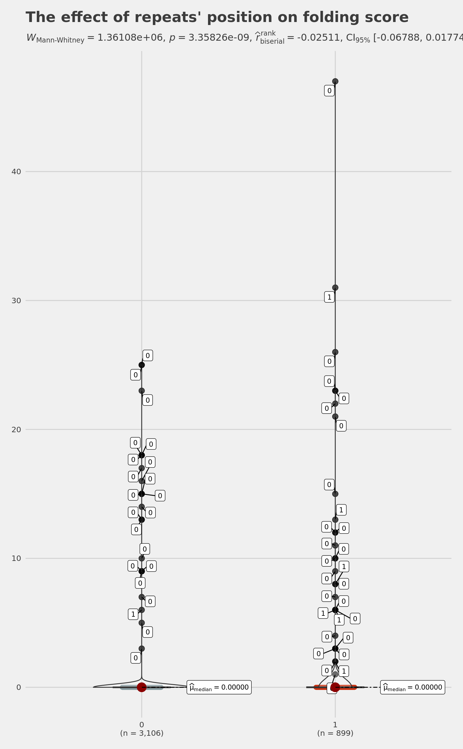

t.test(
  HomologyAndRepeats[HomologyAndRepeats$InfinitySign == 1, ]$GlobalFoldingScore,
  HomologyAndRepeats[HomologyAndRepeats$InfinitySign == 0, ]$GlobalFoldingScore
) # diag 1000: 0.002639

    Welch Two Sample t-test

data:  HomologyAndRepeats[HomologyAndRepeats$InfinitySign == 1, ]$GlobalFoldingScore and HomologyAndRepeats[HomologyAndRepeats$InfinitySign == 0, ]$GlobalFoldingScore
t = 3.0144, df = 1003.9, p-value = 0.002639
alternative hypothesis: true difference in means is not equal to 0
95 percent confidence interval:
 0.1018345 0.4817022
sample estimates:
 mean of x  mean of y 
0.38932147 0.09755312 

pltViolRepFoldingInfSignP <-
  ggbetweenstats(
    data = HomologyAndRepeats,
    x = InfinitySign,
    y = GlobalFoldingScore,
    type = "p",
    # Wilcoxon for two group
    mean.ci = TRUE,
    nboot = 10000,
    # number of iteration for statistical CI
    k = 5,
    # number of decimal places for statistical results
    outlier.tagging = TRUE, # whether outliers need to be tagged
    outlier.label = FirstWindow,
    xlab = '"3D" Position',
    # label for the x-axis variable
    ylab = "in silico folding score",
    # label for the y-axis variable
    title = "The effect of repeats' position on folding score",
    # title text for the plot
    ggtheme = ggthemes::theme_fivethirtyeight(),
    # choosing a different theme
    package = "wesanderson",
    # package from which color palette is to be taken
    palette = "Royal1",
    # choosing a different color palette
    notch = TRUE,
    messages = TRUE
  )
# Note: 95% CI for effect size estimate was computed with 10000 bootstrap samples
# Note: Shapiro-Wilk Normality Test for in silico folding score: p-value = < 0.001
# Note: Bartlett's test for homogeneity of variances for factor "3D" Position: p-value = < 0.001
cowplot::save_plot(
  plot = pltViolRepFoldingInfSignP,
  base_height = 8,
  base_asp = 1.618,
  file = normalizePath(
    file.path(plots_dir, "violin_rep_folding_infsign_p.pdf")
  )
)

pltViolRepFoldingInfSignP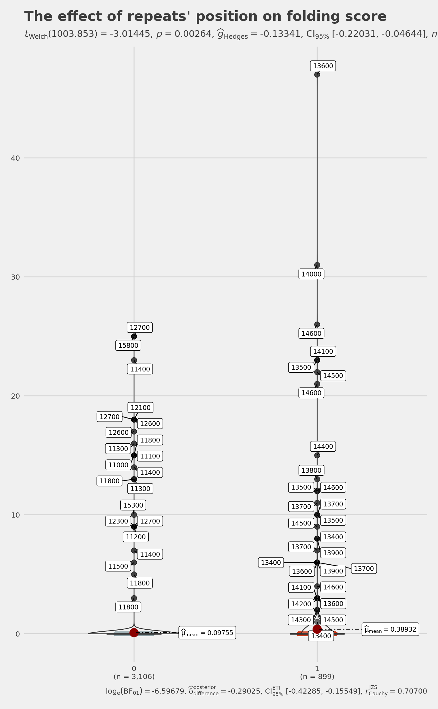

summary(HomologyAndRepeats[HomologyAndRepeats$InfinitySign == 1, ]$GlobalFoldingScore) # diag 1000: 0.3893

   Min. 1st Qu.  Median    Mean 3rd Qu.    Max. 
 0.0000  0.0000  0.0000  0.3893  0.0000 47.0000 

summary(HomologyAndRepeats[HomologyAndRepeats$InfinitySign == 0, ]$GlobalFoldingScore) # diag 1000: 0.09755

    Min.  1st Qu.   Median     Mean  3rd Qu.     Max. 
 0.00000  0.00000  0.00000  0.09755  0.00000 25.00000 

we have to link better global folding and InfinitySign model - till now it was done by eye. Clusterisation? One cluster?

9: LOGISTIC REGRESSION: HomologyAndRepeats\(Deletion as a function of HomologyAndRepeats\)MicroHomologyScore and HomologyAndRepeats$InfinitySign:

a <-
  glm(
    HomologyAndRepeats$Deletion ~ HomologyAndRepeats$MicroHomologyScore + HomologyAndRepeats$InfinitySign,
    family = "binomial"
  )
summary(a)

Call:
glm(formula = HomologyAndRepeats$Deletion ~ HomologyAndRepeats$MicroHomologyScore + 
    HomologyAndRepeats$InfinitySign, family = "binomial")

Deviance Residuals: 
    Min       1Q   Median       3Q      Max  
-1.3434  -0.3920  -0.3293  -0.2893   2.6338  

Coefficients:
                                       Estimate Std. Error z value Pr(>|z|)    
(Intercept)                           -4.573709   0.297535 -15.372  < 2e-16 ***
HomologyAndRepeats$MicroHomologyScore  0.018946   0.003026   6.262  3.8e-10 ***
HomologyAndRepeats$InfinitySign        2.170671   0.106329  20.415  < 2e-16 ***
---
Signif. codes:  0 '***' 0.001 '**' 0.01 '*' 0.05 '.' 0.1 ' ' 1

(Dispersion parameter for binomial family taken to be 1)

    Null deviance: 2924.7  on 4004  degrees of freedom
Residual deviance: 2450.6  on 4002  degrees of freedom
AIC: 2456.6

Number of Fisher Scoring iterations: 5

ggstatsplot::ggcoefstats(a)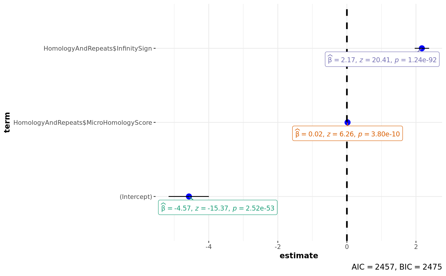

broom::tidy(a)

broom::glance(a)

a <-
  glm(
    HomologyAndRepeats$Deletion ~ scale(HomologyAndRepeats$MicroHomologyScore) + scale(HomologyAndRepeats$InfinitySign),
    family = "binomial"
  )
summary(a) # PAPER!!! 0.33 + 0.91

Call:
glm(formula = HomologyAndRepeats$Deletion ~ scale(HomologyAndRepeats$MicroHomologyScore) + 
    scale(HomologyAndRepeats$InfinitySign), family = "binomial")

Deviance Residuals: 
    Min       1Q   Median       3Q      Max  
-1.3434  -0.3920  -0.3293  -0.2893   2.6338  

Coefficients:
                                             Estimate Std. Error z value
(Intercept)                                  -2.38296    0.06412 -37.167
scale(HomologyAndRepeats$MicroHomologyScore)  0.32592    0.05205   6.262
scale(HomologyAndRepeats$InfinitySign)        0.90579    0.04437  20.415
                                             Pr(>|z|)    
(Intercept)                                   < 2e-16 ***
scale(HomologyAndRepeats$MicroHomologyScore)  3.8e-10 ***
scale(HomologyAndRepeats$InfinitySign)        < 2e-16 ***
---
Signif. codes:  0 '***' 0.001 '**' 0.01 '*' 0.05 '.' 0.1 ' ' 1

(Dispersion parameter for binomial family taken to be 1)

    Null deviance: 2924.7  on 4004  degrees of freedom
Residual deviance: 2450.6  on 4002  degrees of freedom
AIC: 2456.6

Number of Fisher Scoring iterations: 5

ggstatsplot::ggcoefstats(a)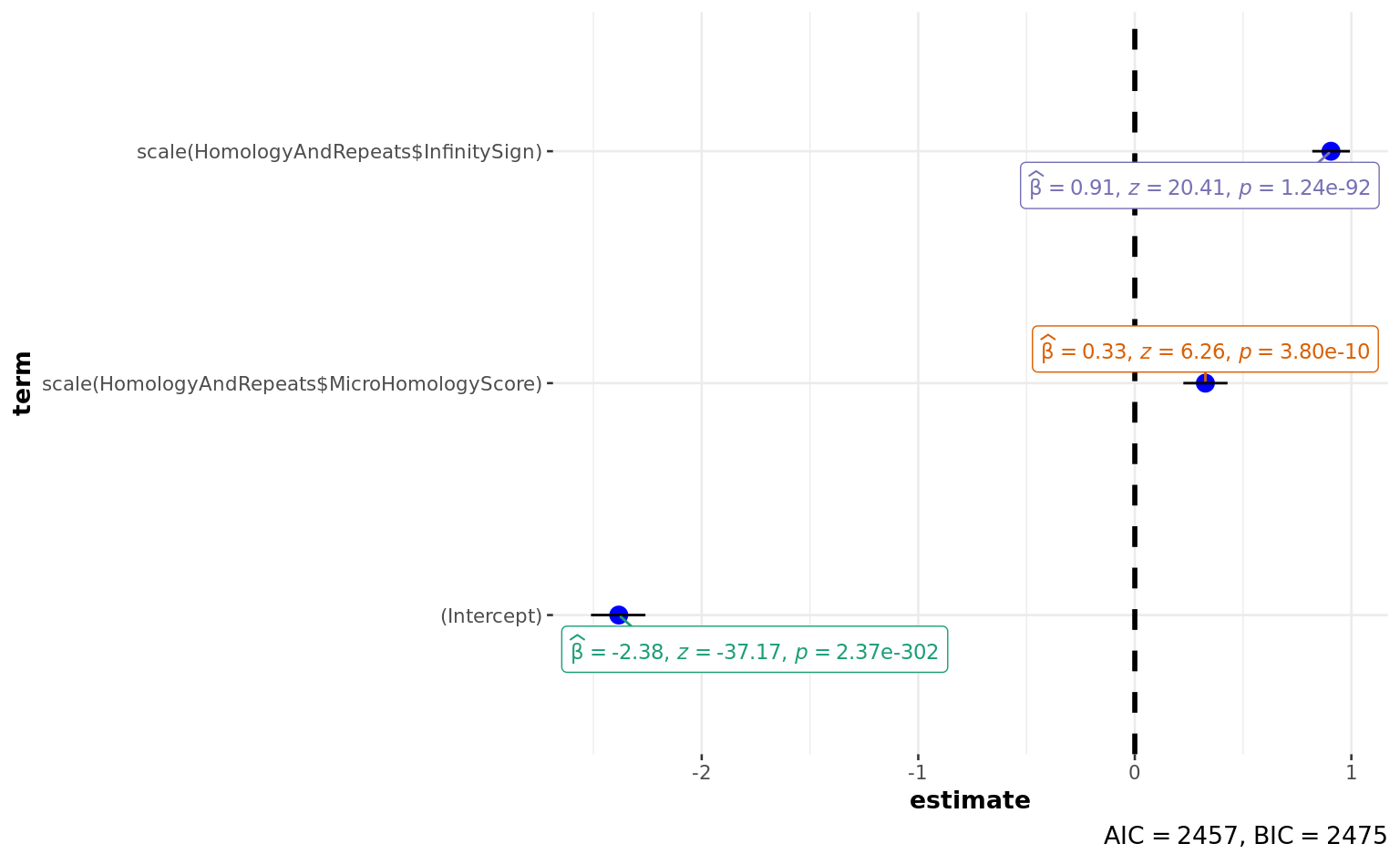

broom::tidy(a)

broom::glance(a)

a <-
  glm(
    HomologyAndRepeats$Deletion ~ HomologyAndRepeats$MicroHomologyScore + HomologyAndRepeats$GlobalFoldingScore,
    family = "binomial"
  )
summary(a) # non significant - may be I have to take it on bigger scale! (1kb without diagonal, because this is global parameter not precise)

Call:
glm(formula = HomologyAndRepeats$Deletion ~ HomologyAndRepeats$MicroHomologyScore + 
    HomologyAndRepeats$GlobalFoldingScore, family = "binomial")

Deviance Residuals: 
    Min       1Q   Median       3Q      Max  
-0.8482  -0.5288  -0.4803  -0.4322   2.4455  

Coefficients:
                                       Estimate Std. Error z value Pr(>|z|)    
(Intercept)                           -3.570891   0.266681 -13.390  < 2e-16 ***
HomologyAndRepeats$MicroHomologyScore  0.017085   0.002793   6.117 9.54e-10 ***
HomologyAndRepeats$GlobalFoldingScore  0.005585   0.028785   0.194    0.846    
---
Signif. codes:  0 '***' 0.001 '**' 0.01 '*' 0.05 '.' 0.1 ' ' 1

(Dispersion parameter for binomial family taken to be 1)

    Null deviance: 2924.7  on 4004  degrees of freedom
Residual deviance: 2887.5  on 4002  degrees of freedom
AIC: 2893.5

Number of Fisher Scoring iterations: 4

# to reconstruct 100 bp matrix back from 1 kb matrix!!!!!
ggstatsplot::ggcoefstats(a)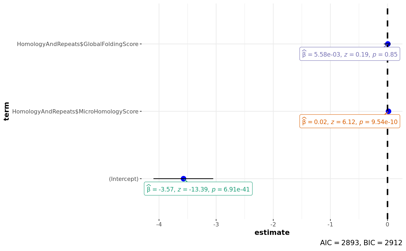

broom::tidy(a)

broom::glance(a)

get residuals and correlate them with global matrix

a <-
  glm(HomologyAndRepeats$Deletion ~ HomologyAndRepeats$MicroHomologyScore,
      family = "binomial"
  )
ggstatsplot::ggcoefstats(a)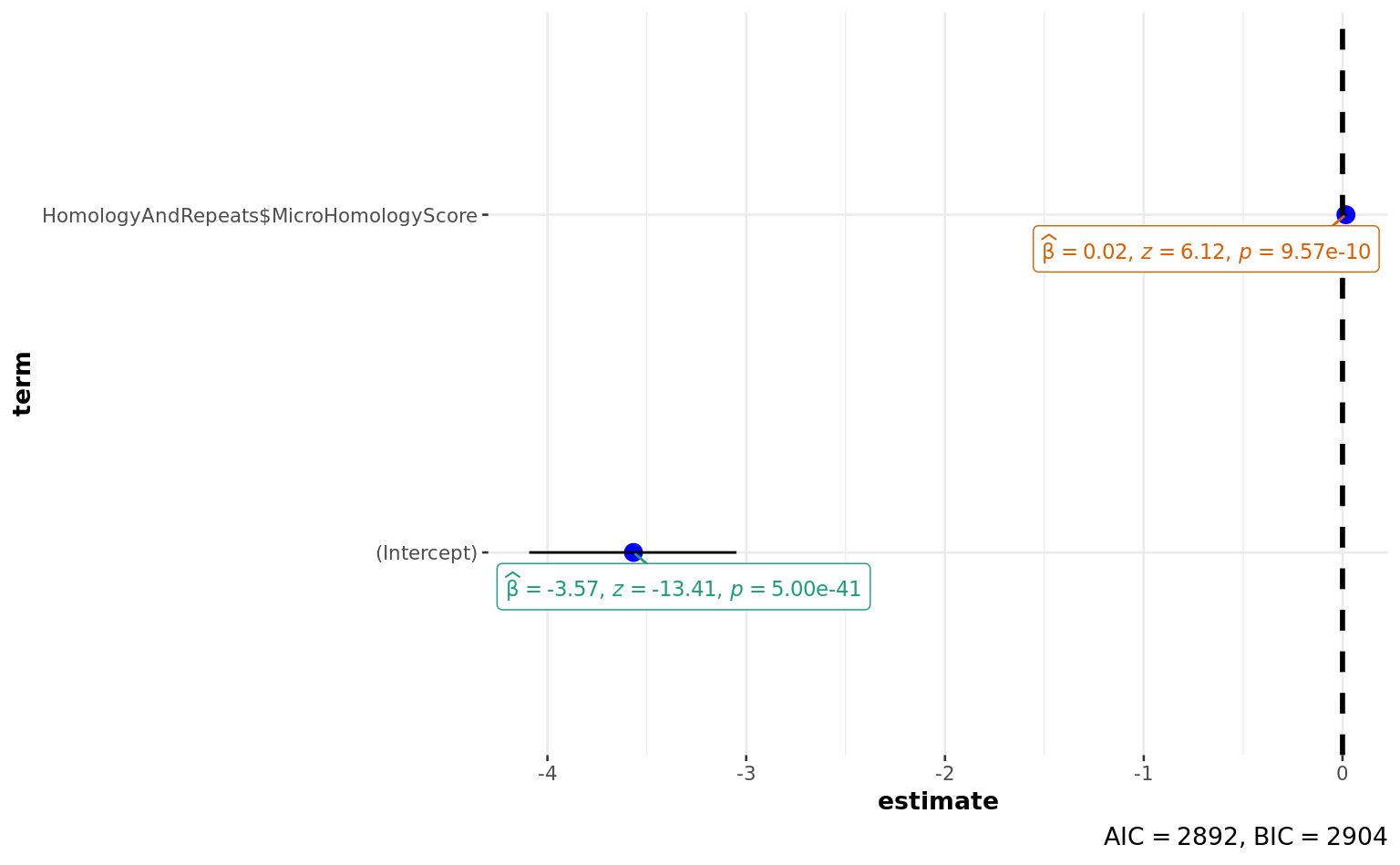

HomologyAndRepeats$Residuals <- residuals(a)
summary(HomologyAndRepeats$Residuals)

   Min. 1st Qu.  Median    Mean 3rd Qu.    Max. 
-0.8477 -0.5290 -0.4805 -0.1950 -0.4290  2.4445 

pspearman::spearman.test(
  HomologyAndRepeats$Residuals,
  HomologyAndRepeats$GlobalFoldingScore
)

    Spearman's rank correlation rho

data:  HomologyAndRepeats$Residuals and HomologyAndRepeats$GlobalFoldingScore
S = 1.0104e+10, p-value = 0.0003666
alternative hypothesis: true rho is not equal to 0
sample estimates:
       rho 
0.05628272 

reconstruct Global folding 100 bp back from 1kb resolution (GlobalFolding1000) assuming that global folding can work remotely enough.

another idea - to use a distance from a given cell to closest contact (from global matrix) - so, infinity sign is not zero or one, but continuos!

HomologyAndRepeats$FirstWindowWholeKbRes <-
  round(HomologyAndRepeats$FirstWindow, -3)
HomologyAndRepeats$SecondWindowWholeKbRes <-
  round(HomologyAndRepeats$SecondWindow, -3)
janitor::tabyl(
  HomologyAndRepeats,
  FirstWindowWholeKbRes,
  SecondWindowWholeKbRes
)

HomologyAndRepeats <- merge(
  HomologyAndRepeats,
  GlobalFolding1000,
  by = c("FirstWindowWholeKbRes", "SecondWindowWholeKbRes")
)

a <-
  glm(
    HomologyAndRepeats$Deletion ~ scale(HomologyAndRepeats$MicroHomologyScore) + scale(HomologyAndRepeats$GlobalFolding1000Score),
    family = "binomial"
  )
summary(a)

Call:
glm(formula = HomologyAndRepeats$Deletion ~ scale(HomologyAndRepeats$MicroHomologyScore) + 
    scale(HomologyAndRepeats$GlobalFolding1000Score), family = "binomial")

Deviance Residuals: 
    Min       1Q   Median       3Q      Max  
-0.8795  -0.5271  -0.4791  -0.4281   2.4577  

Coefficients:
                                                 Estimate Std. Error z value
(Intercept)                                      -2.03721    0.05031 -40.490
scale(HomologyAndRepeats$MicroHomologyScore)      0.29126    0.04806   6.061
scale(HomologyAndRepeats$GlobalFolding1000Score)  0.09128    0.04444   2.054
                                                 Pr(>|z|)    
(Intercept)                                       < 2e-16 ***
scale(HomologyAndRepeats$MicroHomologyScore)     1.35e-09 ***
scale(HomologyAndRepeats$GlobalFolding1000Score)     0.04 *  
---
Signif. codes:  0 '***' 0.001 '**' 0.01 '*' 0.05 '.' 0.1 ' ' 1

(Dispersion parameter for binomial family taken to be 1)

    Null deviance: 2924.7  on 4004  degrees of freedom
Residual deviance: 2883.5  on 4002  degrees of freedom
AIC: 2889.5

Number of Fisher Scoring iterations: 5

ggstatsplot::ggcoefstats(a)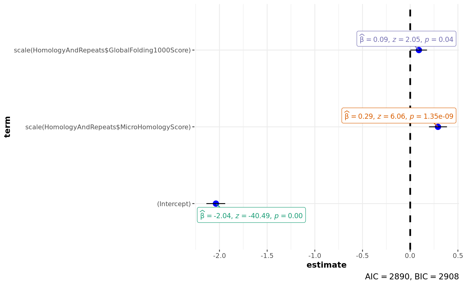

broom::tidy(a) %>%
  kableExtra::kbl() %>%
  kableExtra::kable_styling(
    bootstrap_options = c(
      "bordered", "condensed", "responsive", "striped"
    )
  )

term	estimate	std.error	statistic	p.value
(Intercept)	-2.0372126	0.0503135	-40.490337	0.0000000
scale(HomologyAndRepeats\(MicroHomologyScore) </td> <td style="text-align:right;"> 0.2912598 </td> <td style="text-align:right;"> 0.0480566 </td> <td style="text-align:right;"> 6.060761 </td> <td style="text-align:right;"> 0.0000000 </td> </tr> <tr> <td style="text-align:left;"> scale(HomologyAndRepeats\)GlobalFolding1000Score)	0.0912813	0.0444382	2.054118	0.0399643

broom::glance(a) %>%
  kableExtra::kbl() %>%
  kableExtra::kable_styling(
    bootstrap_options = c(
      "bordered", "condensed", "responsive", "striped"
    )
  )

null.deviance	df.null	logLik	AIC	BIC	deviance	df.residual	nobs
2924.693	4004	-1441.768	2889.536	2908.422	2883.536	4002	4005

derive distance to the strongest contact: 6500 vs 14500 (see heatmap: global folding 1 kb resolution)

HomologyAndRepeats$DistanceToContact <- 0
for (i in seq_len(nrow(HomologyAndRepeats))) {
  # i = 1
  HomologyAndRepeats$DistanceToContact[i] <- raster::pointDistance(
    c(
      HomologyAndRepeats$FirstWindow[i],
      HomologyAndRepeats$SecondWindow[i]
    ),
    c(14550, 6550),
    lonlat = FALSE
  )
}

skim(HomologyAndRepeats$DistanceToContact) %>%
  kableExtra::kbl() %>%
  kableExtra::kable_styling(
    bootstrap_options = c(
      "bordered", "condensed", "responsive", "striped"
    )
  )

skim_type	skim_variable	n_missing	complete_rate	numeric.mean	numeric.sd	numeric.p0	numeric.p25	numeric.p50	numeric.p75	numeric.p100	numeric.hist
numeric	data	0	1	3726.984	1747.957	70.71068	2392.697	3842.525	4962.358	8245.302	▃▆▇▅▁

# the closest: -70; the most distant: -8245

a <-
  glm(
    HomologyAndRepeats$Deletion ~ scale(HomologyAndRepeats$MicroHomologyScore) + scale(HomologyAndRepeats$DistanceToContact),
    family = "binomial"
  )
summary(a)

Call:
glm(formula = HomologyAndRepeats$Deletion ~ scale(HomologyAndRepeats$MicroHomologyScore) + 
    scale(HomologyAndRepeats$DistanceToContact), family = "binomial")

Deviance Residuals: 
    Min       1Q   Median       3Q      Max  
-1.3824  -0.5088  -0.3101  -0.1852   3.0099  

Coefficients:
                                             Estimate Std. Error z value
(Intercept)                                  -2.56654    0.07383 -34.760
scale(HomologyAndRepeats$MicroHomologyScore)  0.43224    0.05269   8.203
scale(HomologyAndRepeats$DistanceToContact)  -1.24881    0.06520 -19.152
                                             Pr(>|z|)    
(Intercept)                                   < 2e-16 ***
scale(HomologyAndRepeats$MicroHomologyScore) 2.34e-16 ***
scale(HomologyAndRepeats$DistanceToContact)   < 2e-16 ***
---
Signif. codes:  0 '***' 0.001 '**' 0.01 '*' 0.05 '.' 0.1 ' ' 1

(Dispersion parameter for binomial family taken to be 1)

    Null deviance: 2924.7  on 4004  degrees of freedom
Residual deviance: 2402.3  on 4002  degrees of freedom
AIC: 2408.3

Number of Fisher Scoring iterations: 6

ggstatsplot::ggcoefstats(a)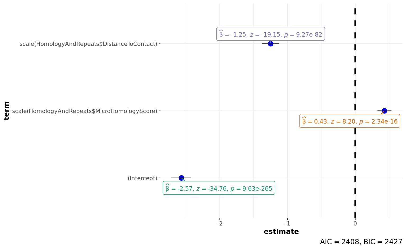

broom::tidy(a) %>%
  kableExtra::kbl() %>%
  kableExtra::kable_styling(
    bootstrap_options = c(
      "bordered", "condensed", "responsive", "striped"
    )
  )

term	estimate	std.error	statistic	p.value
(Intercept)	-2.566536	0.0738349	-34.76046	0
scale(HomologyAndRepeats\(MicroHomologyScore) </td> <td style="text-align:right;"> 0.432243 </td> <td style="text-align:right;"> 0.0526914 </td> <td style="text-align:right;"> 8.20330 </td> <td style="text-align:right;"> 0 </td> </tr> <tr> <td style="text-align:left;"> scale(HomologyAndRepeats\)DistanceToContact)	-1.248810	0.0652043	-19.15226	0

broom::glance(a) %>%
  kableExtra::kbl() %>%
  kableExtra::kable_styling(
    bootstrap_options = c(
      "bordered", "condensed", "responsive", "striped"
    )
  )

null.deviance	df.null	logLik	AIC	BIC	deviance	df.residual	nobs
2924.693	4004	-1201.136	2408.272	2427.158	2402.272	4002	4005

derive distance to the common repeat:

HomologyAndRepeats$DistanceToContact <- 0
for (i in seq_len(nrow(HomologyAndRepeats))) {
  # i = 1
  HomologyAndRepeats$DistanceToContact[i] <- pointDistance(
    c(
      HomologyAndRepeats$FirstWindow[i],
      HomologyAndRepeats$SecondWindow[i]
    ),
    c(13447, 8469),
    lonlat = FALSE
  ) #  (8469-8482 - 13447-13459)
}
skim(HomologyAndRepeats$DistanceToContact) %>%
  kableExtra::kbl() %>%
  kableExtra::kable_styling(
    bootstrap_options = c(
      "bordered", "condensed", "responsive", "striped"
    )
  )

skim_type	skim_variable	n_missing	complete_rate	numeric.mean	numeric.sd	numeric.p0	numeric.p25	numeric.p50	numeric.p75	numeric.p100	numeric.hist
numeric	data	0	1	2744.767	1354.259	56.30275	1783.359	2535.62	3547.897	6939.998	▃▇▅▂▁

a <-
  glm(
    HomologyAndRepeats$Deletion ~ scale(HomologyAndRepeats$MicroHomologyScore) + scale(HomologyAndRepeats$DistanceToContact),
    family = "binomial"
  )
summary(a)

Call:
glm(formula = HomologyAndRepeats$Deletion ~ scale(HomologyAndRepeats$MicroHomologyScore) + 
    scale(HomologyAndRepeats$DistanceToContact), family = "binomial")

Deviance Residuals: 
    Min       1Q   Median       3Q      Max  
-1.2894  -0.5524  -0.3985  -0.2235   2.8234  

Coefficients:
                                             Estimate Std. Error z value
(Intercept)                                  -2.35793    0.06536 -36.077
scale(HomologyAndRepeats$MicroHomologyScore)  0.27667    0.05038   5.492
scale(HomologyAndRepeats$DistanceToContact)  -1.00602    0.06878 -14.627
                                             Pr(>|z|)    
(Intercept)                                   < 2e-16 ***
scale(HomologyAndRepeats$MicroHomologyScore) 3.98e-08 ***
scale(HomologyAndRepeats$DistanceToContact)   < 2e-16 ***
---
Signif. codes:  0 '***' 0.001 '**' 0.01 '*' 0.05 '.' 0.1 ' ' 1

(Dispersion parameter for binomial family taken to be 1)

    Null deviance: 2924.7  on 4004  degrees of freedom
Residual deviance: 2609.1  on 4002  degrees of freedom
AIC: 2615.1

Number of Fisher Scoring iterations: 6

ggstatsplot::ggcoefstats(a)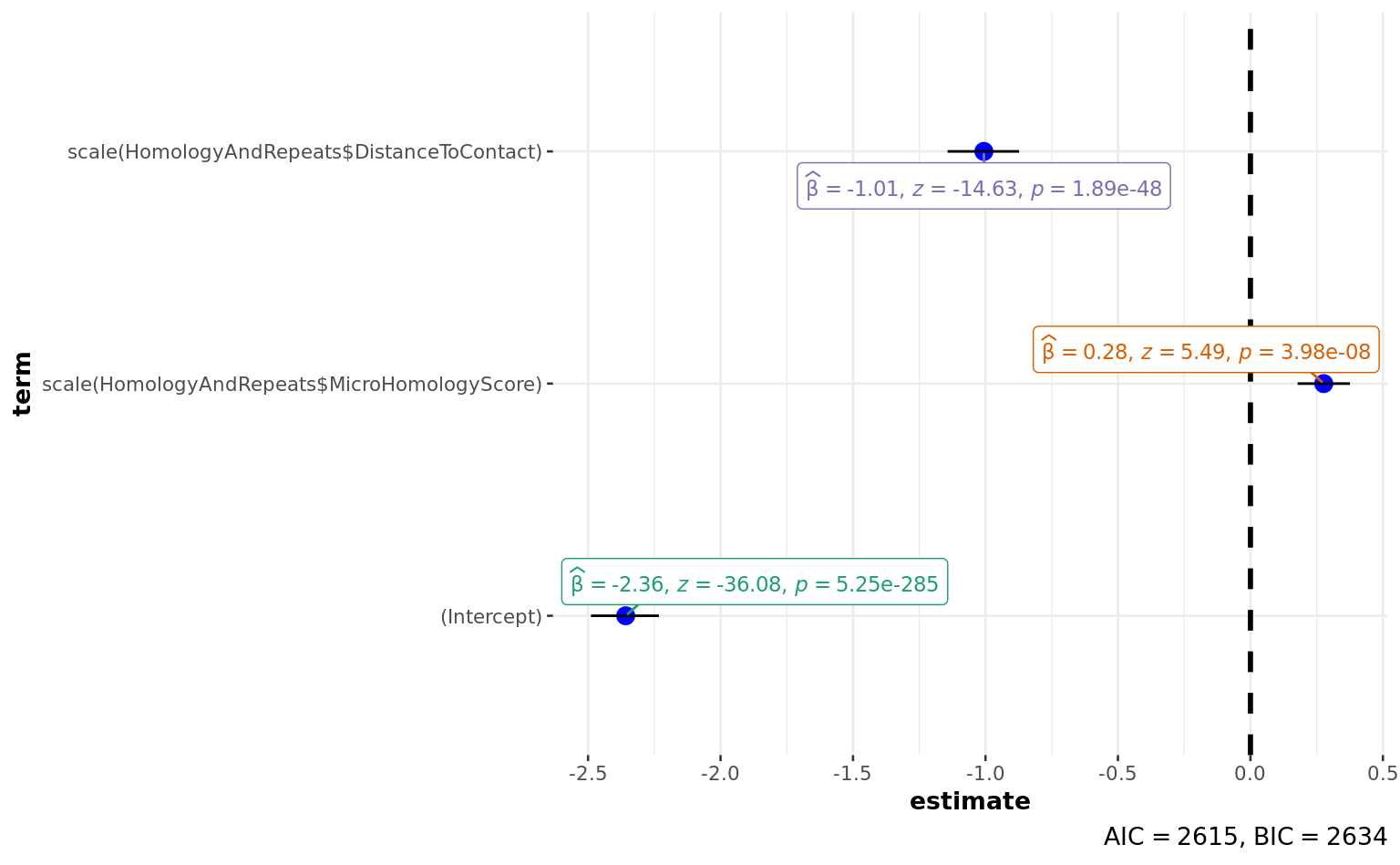 

broom::tidy(a) %>%
  kableExtra::kbl() %>%
  kableExtra::kable_styling(
    bootstrap_options = c(
      "bordered", "condensed", "responsive", "striped"
    )
  )

term	estimate	std.error	statistic	p.value
(Intercept)	-2.3579307	0.0653587	-36.076742	0
scale(HomologyAndRepeats\(MicroHomologyScore) </td> <td style="text-align:right;"> 0.2766745 </td> <td style="text-align:right;"> 0.0503802 </td> <td style="text-align:right;"> 5.491729 </td> <td style="text-align:right;"> 0 </td> </tr> <tr> <td style="text-align:left;"> scale(HomologyAndRepeats\)DistanceToContact)	-1.0060227	0.0687794	-14.626799	0

broom::glance(a) %>%
  kableExtra::kbl() %>%
  kableExtra::kable_styling(
    bootstrap_options = c(
      "bordered", "condensed", "responsive", "striped"
    )
  )

null.deviance	df.null	logLik	AIC	BIC	deviance	df.residual	nobs
2924.693	4004	-1304.572	2615.144	2634.03	2609.144	4002	4005

10: run many logistic regression in the loop and find the Contact Point/zone with the best AIC

mod_fun <- function(Coord1, Coord2) {
  TempDF <-
    HomologyAndRepeats %>%
    dplyr::select(
      FirstWindow,
      SecondWindow,
      Deletion,
      MicroHomologyScore
    ) %>%
    mutate(TempDistanceToContact = purrr::map2_dbl(
      FirstWindow,
      SecondWindow,
      ~ raster::pointDistance(c(.x, .y),
                              c(
                                Coord1,
                                Coord2
                              ),
                              lonlat = F
      )
    ))
  a <-
    glm(
      TempDF$Deletion ~ scale(TempDF$MicroHomologyScore) + scale(TempDF$TempDistanceToContact),
      family = "binomial"
    )
  return(a)
}

Results <- HomologyAndRepeats %>%
  mutate(
    LogRegr.ContactPoint.Coord1 = FirstWindow + 50,
    LogRegr.ContactPoint.Coord2 = SecondWindow + 50
  ) %>%
  mutate(model = furrr::future_map2(
    LogRegr.ContactPoint.Coord1,
    LogRegr.ContactPoint.Coord2,
    mod_fun
  ))

ResultsTidy <- Results$model %>% purrr::map_dfr(~ broom::tidy(.x)[3, ])
ResultsGlance <- Results$model %>% purrr::map_dfr(broom::glance)

HomologyAndRepeats$LogRegr.ContactPoint.PiValue <- ResultsTidy$p.value
HomologyAndRepeats$LogRegr.ContactPoint.Coeff <- ResultsTidy$estimate
HomologyAndRepeats$LogRegr.ContactPoint.AIC <- ResultsGlance$AIC
HomologyAndRepeats$LogRegr.ContactPoint.ResidualDeviance <- ResultsGlance$deviance
HomologyAndRepeats$LogRegr.ContactPoint.Coord1 <- Results$LogRegr.ContactPoint.Coord1
HomologyAndRepeats$LogRegr.ContactPoint.Coord2 <- Results$LogRegr.ContactPoint.Coord2

rm(Results, ResultsGlance, ResultsTidy)
invisible(gc())

write.table(
  HomologyAndRepeats,
  here(plots_dir, "SlipAndJump.HomologyAndRepeats.txt") %>%
    normalizePath(),
  sep = "\t"
)

HomologyAndRepeats <- read.table(
  here(plots_dir, "SlipAndJump.HomologyAndRepeats.txt") %>%
    normalizePath(),
  sep = "\t"
)

HomologyAndRepeats <- HomologyAndRepeats[order(HomologyAndRepeats$LogRegr.ContactPoint.AIC), ]
names(HomologyAndRepeats)

 [1] "FirstWindowWholeKbRes"                
 [2] "SecondWindowWholeKbRes"               
 [3] "FirstWindow"                          
 [4] "SecondWindow"                         
 [5] "DirectRepeatsDensity"                 
 [6] "MicroHomologyScore"                   
 [7] "Deletion"                             
 [8] "InfinitySign"                         
 [9] "InvRepDensScore"                      
[10] "GlobalFoldingScore"                   
[11] "Residuals"                            
[12] "GlobalFolding1000Score"               
[13] "DistanceToContact"                    
[14] "LogRegr.ContactPoint.PiValue"         
[15] "LogRegr.ContactPoint.Coeff"           
[16] "LogRegr.ContactPoint.AIC"             
[17] "LogRegr.ContactPoint.ResidualDeviance"
[18] "LogRegr.ContactPoint.Coord1"          
[19] "LogRegr.ContactPoint.Coord2"          

summary(HomologyAndRepeats$LogRegr.ContactPoint.ResidualDeviance)

   Min. 1st Qu.  Median    Mean 3rd Qu.    Max. 
   2307    2692    2848    2756    2879    2888 

summary(HomologyAndRepeats$LogRegr.ContactPoint.AIC)

   Min. 1st Qu.  Median    Mean 3rd Qu.    Max. 
   2313    2698    2854    2762    2885    2894 

HomologyAndRepeats %>% skim()

Data summary

Name	Piped data
Number of rows	4005
Number of columns	19
_______________________
Column type frequency:
numeric	19
________________________
Group variables	None

Variable type: numeric

skim_variable	n_missing	complete_rate	mean	sd	p0	p25	p50	p75	p100	hist
FirstWindowWholeKbRes	0	1	12879.15	2148.55	7000.00	11000.00	13000.00	15000.00	16000.00	▁▃▆▇▆
SecondWindowWholeKbRes	0	1	8821.22	2144.50	6000.00	7000.00	8000.00	10000.00	15000.00	▇▇▆▃▁
FirstWindow	0	1	12866.67	2109.50	7000.00	11400.00	13200.00	14700.00	15800.00	▁▃▅▆▇
SecondWindow	0	1	8833.33	2109.50	5900.00	7000.00	8500.00	10300.00	14700.00	▇▆▅▃▁
DirectRepeatsDensity	0	1	5.77	7.79	0.00	0.00	0.00	10.00	57.00	▇▂▁▁▁
MicroHomologyScore	0	1	89.91	17.20	27.00	79.00	89.00	100.00	160.00	▁▅▇▂▁
Deletion	0	1	0.12	0.32	0.00	0.00	0.00	0.00	1.00	▇▁▁▁▁
InfinitySign	0	1	0.22	0.42	0.00	0.00	0.00	0.00	1.00	▇▁▁▁▂
InvRepDensScore	0	1	1.39	3.81	0.00	0.00	0.00	0.00	31.00	▇▁▁▁▁
GlobalFoldingScore	0	1	0.16	1.74	0.00	0.00	0.00	0.00	47.00	▇▁▁▁▁
Residuals	0	1	-0.20	0.83	-0.85	-0.53	-0.48	-0.43	2.44	▇▁▁▁▁
GlobalFolding1000Score	0	1	15.41	37.87	0.00	0.00	0.00	0.00	173.00	▇▁▁▁▁
DistanceToContact	0	1	2744.77	1354.26	56.30	1783.36	2535.62	3547.90	6940.00	▃▇▅▂▁
LogRegr.ContactPoint.PiValue	0	1	0.07	0.18	0.00	0.00	0.00	0.00	1.00	▇▁▁▁▁
LogRegr.ContactPoint.Coeff	0	1	-0.31	0.60	-1.51	-0.81	-0.10	0.17	0.46	▃▂▂▅▇
LogRegr.ContactPoint.AIC	0	1	2762.23	179.48	2313.25	2697.87	2853.59	2885.22	2893.52	▁▁▁▁▇
LogRegr.ContactPoint.ResidualDeviance	0	1	2756.23	179.48	2307.25	2691.87	2847.59	2879.22	2887.52	▁▁▁▁▇
LogRegr.ContactPoint.Coord1	0	1	12916.67	2109.50	7050.00	11450.00	13250.00	14750.00	15850.00	▁▃▅▆▇
LogRegr.ContactPoint.Coord2	0	1	8883.33	2109.50	5950.00	7050.00	8550.00	10350.00	14750.00	▇▆▅▃▁

temp <- HomologyAndRepeats[
  HomologyAndRepeats$LogRegr.ContactPoint.Coord1 == 11950 &
    HomologyAndRepeats$LogRegr.ContactPoint.Coord2 == 8950,
]
temp

Heatmap merged microhomology and AIC scores

tib <- HomologyAndRepeats %>%
  dplyr::select(
    LogRegr.ContactPoint.Coord1,
    LogRegr.ContactPoint.Coord2,
    MicroHomologyScore,
    LogRegr.ContactPoint.AIC
  ) %>%
  ggasym::asymmetrise(
    .,
    LogRegr.ContactPoint.Coord1,
    LogRegr.ContactPoint.Coord2
  )

pltHeatmap_mhAIC <- ggplot(
  tib,
  aes(
    x = LogRegr.ContactPoint.Coord1,
    y = LogRegr.ContactPoint.Coord2
  )
) +
  geom_asymmat(aes(
    fill_br = LogRegr.ContactPoint.AIC,
    fill_tl = MicroHomologyScore
  )) +
  scale_fill_br_distiller(
    type = "seq",
    palette = "Spectral",
    direction = 1,
    na.value = "white",
    guide = guide_colourbar(
      direction = "horizontal",
      order = 1,
      title.position = "top"
    )
  ) +
  scale_fill_tl_distiller(
    type = "seq",
    palette = "RdYlGn",
    direction = 1,
    na.value = "white",
    guide = guide_colourbar(
      direction = "horizontal",
      order = 2,
      title.position = "top"
    )
  ) +
  labs(
    fill_br = "top-right Contact AIC",
    fill_tl = "bottom-left Microhomology",
    title = "Model of mtDNA contacts"
  ) +
  theme_bw() +
  theme(
    axis.title = element_blank(),
    plot.title = element_text(hjust = 0.5),
    panel.background = element_rect(fill = "white"),
    panel.grid = element_blank()
  )

cowplot::save_plot(
  plot = pltHeatmap_mhAIC,
  base_height = 8.316,
  base_width = 11.594,
  file = normalizePath(
    file.path(plots_dir, "heatmap_microhomology_AIC.pdf")
  )
)

pltHeatmap_mhAIC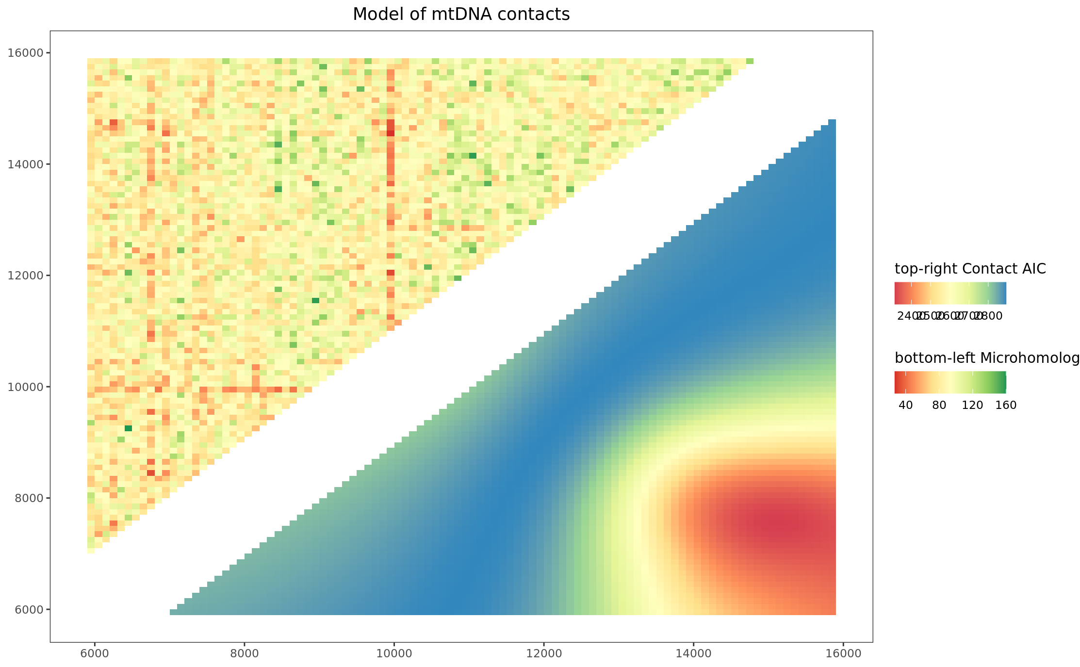

Article version Figure 2C: Heatmap merged microhomology and AIC scores with actual deletions circles

tib <- HomologyAndRepeats %>%
  dplyr::select(
    LogRegr.ContactPoint.Coord1,
    LogRegr.ContactPoint.Coord2,
    MicroHomologyScore,
    LogRegr.ContactPoint.AIC,
    Deletion
  ) %>%
  asymmetrise(
    .,
    LogRegr.ContactPoint.Coord1,
    LogRegr.ContactPoint.Coord2
  )

pltHeatmap_mhAIC_wt_deletions <- ggplot(
  tib,
  aes(
    x = LogRegr.ContactPoint.Coord1,
    y = LogRegr.ContactPoint.Coord2
  )
) +
  geom_asymmat(aes(
    fill_br = LogRegr.ContactPoint.AIC,
    fill_tl = MicroHomologyScore
  )) +
  geom_point(
    data = subset(tib, Deletion > 0),
    aes(alpha = 0.3),
    shape = 1,
    size = 2.3,
    color = "#d73027", # "#041c00",
    show.legend = FALSE,
    na.rm = TRUE
  ) +
  scale_fill_br_gradientn(
    colours = viridis::viridis(2000)[250:2000],
    na.value = "white",
    guide = guide_colourbar(
      direction = "horizontal",
      order = 1,
      title.position = "top",
      barwidth = 10, barheight = 1
    )
  ) +
  scale_fill_tl_distiller(
    type = "div",
    palette = "RdYlBu",
    direction = 1,
    na.value = "white",
    guide = guide_colourbar(
      direction = "horizontal",
      order = 2,
      title.position = "top",
      barwidth = 10, barheight = 1
    )
  ) +
  labs(
    fill_br = "top-right Contact AIC",
    fill_tl = "bottom-left Microhomology",
    title = "Model of mtDNA contacts and deletions"
  ) +
  theme_bw() +
  theme(
    axis.title = element_blank(),
    plot.title = element_text(hjust = 0.5),
    panel.background = element_rect(fill = "white"),
    panel.grid = element_blank(),
    legend.position = "bottom",
    legend.box = "horizontal"
  )


cowplot::save_plot(
  plot = pltHeatmap_mhAIC_wt_deletions,
  base_height = 8.316,
  base_asp = 0.9,
  file = normalizePath(
    file.path(plots_dir, "heatmap_microhomology_AIC_wt_deledions.svg")
  )
)

pltHeatmap_mhAIC_wt_deletions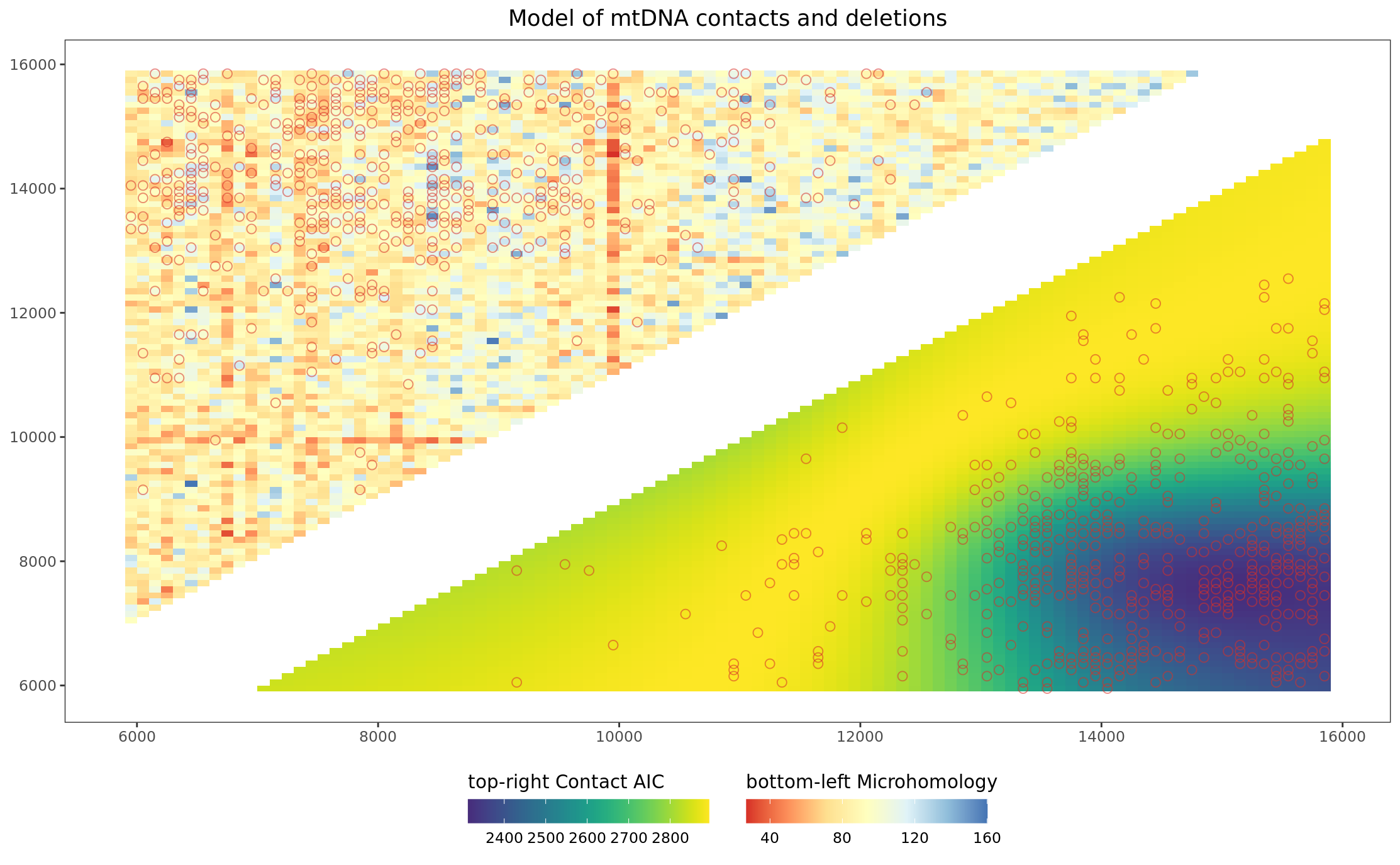

Figures 2C-D:

pltHeatmap_mhAIC_wt_deletions | gg_bind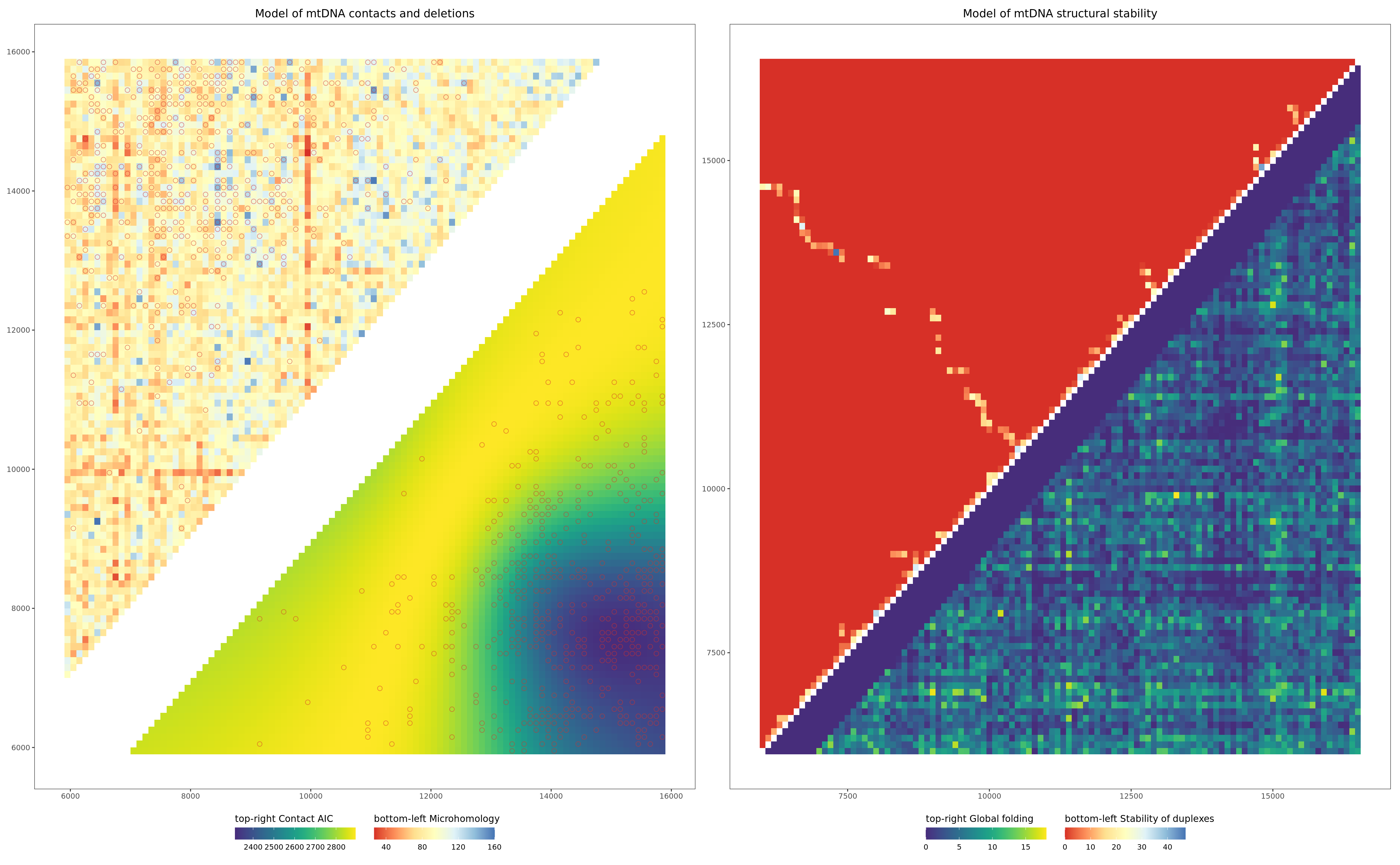

Session information

sessionInfo()

R version 4.2.2 (2022-10-31)
Platform: x86_64-pc-linux-gnu (64-bit)
Running under: Ubuntu 22.04.1 LTS

Matrix products: default
BLAS:   /usr/lib/x86_64-linux-gnu/openblas-pthread/libblas.so.3
LAPACK: /usr/lib/x86_64-linux-gnu/openblas-pthread/libopenblasp-r0.3.20.so

locale:
 [1] LC_CTYPE=en_US.UTF-8       LC_NUMERIC=C              
 [3] LC_TIME=en_US.UTF-8        LC_COLLATE=en_US.UTF-8    
 [5] LC_MONETARY=en_US.UTF-8    LC_MESSAGES=en_US.UTF-8   
 [7] LC_PAPER=en_US.UTF-8       LC_NAME=C                 
 [9] LC_ADDRESS=C               LC_TELEPHONE=C            
[11] LC_MEASUREMENT=en_US.UTF-8 LC_IDENTIFICATION=C       

attached base packages:
[1] stats     graphics  grDevices datasets  utils     methods   base     

other attached packages:
 [1] ggasym_0.1.6       ggstatsplot_0.11.0 pspearman_0.3-1    skimr_2.1.5       
 [5] raster_3.6-20      sp_1.6-0           patchwork_1.1.2    cowplot_1.1.1     
 [9] furrr_0.3.1        future_1.32.0      here_1.0.1         lubridate_1.9.2   
[13] forcats_1.0.0      stringr_1.5.0      dplyr_1.1.1        purrr_1.0.1       
[17] readr_2.1.4        tidyr_1.3.0        tibble_3.2.1       ggplot2_3.4.2     
[21] tidyverse_2.0.0    reshape2_1.4.4     workflowr_1.7.0   

loaded via a namespace (and not attached):
  [1] colorspace_2.1-0       sjlabelled_1.2.0       rprojroot_2.0.3       
  [4] snakecase_0.11.0       parameters_0.20.2      base64enc_0.1-3       
  [7] fs_1.6.1               rstudioapi_0.14        listenv_0.9.0         
 [10] farver_2.1.1           MatrixModels_0.5-1     ggrepel_0.9.3         
 [13] mvtnorm_1.1-3          fansi_1.0.4            xml2_1.3.3            
 [16] codetools_0.2-19       cachem_1.0.7           knitr_1.42            
 [19] sjmisc_2.8.9           zeallot_0.1.0          jsonlite_1.8.4        
 [22] broom_1.0.4            effectsize_0.8.3       compiler_4.2.2        
 [25] httr_1.4.5             backports_1.4.1        Matrix_1.5-3          
 [28] fastmap_1.1.1          cli_3.6.1              later_1.3.0           
 [31] htmltools_0.5.5        tools_4.2.2            coda_0.19-4           
 [34] gtable_0.3.3           glue_1.6.2             ggthemes_4.2.4        
 [37] Rcpp_1.0.10            jquerylib_0.1.4        vctrs_0.6.1           
 [40] svglite_2.1.1          insight_0.19.1         xfun_0.38             
 [43] globals_0.16.2         ps_1.7.4               rvest_1.0.3           
 [46] timechange_0.2.0       lifecycle_1.0.3        renv_0.17.2           
 [49] terra_1.7-18           getPass_0.2-2          MASS_7.3-58.1         
 [52] scales_1.2.1           BayesFactor_0.9.12-4.4 ragg_1.2.5            
 [55] hms_1.1.3              promises_1.2.0.1       parallel_4.2.2        
 [58] rematch2_2.1.2         RColorBrewer_1.1-3     prismatic_1.1.1       
 [61] yaml_2.3.7             pbapply_1.7-0          gridExtra_2.3         
 [64] sass_0.4.5             stringi_1.7.12         paletteer_1.5.0       
 [67] highr_0.10             bayestestR_0.13.0      repr_1.1.6            
 [70] rlang_1.1.0            pkgconfig_2.0.3        systemfonts_1.0.4     
 [73] evaluate_0.20          lattice_0.20-45        labeling_0.4.2        
 [76] processx_3.8.0         tidyselect_1.2.0       parallelly_1.35.0     
 [79] plyr_1.8.8             magrittr_2.0.3         R6_2.5.1              
 [82] generics_0.1.3         pillar_1.9.0           whisker_0.4.1         
 [85] withr_2.5.0            datawizard_0.7.1       performance_0.10.2    
 [88] janitor_2.2.0          utf8_1.2.3             correlation_0.8.3     
 [91] tzdb_0.3.0             rmarkdown_2.21         viridis_0.6.2         
 [94] grid_4.2.2             callr_3.7.3            git2r_0.31.0          
 [97] webshot_0.5.4          digest_0.6.31          httpuv_1.6.9          
[100] textshaping_0.3.6      statsExpressions_1.5.0 munsell_0.5.0         
[103] kableExtra_1.3.4       viridisLite_0.4.1      bslib_0.4.2